Statistical Policing
Goals
In shared network environments, excessive traffic from misbehaving sources can disrupt other applications by consuming bandwidth meant for well-behaved traffic. When multiple clients share the same network infrastructure, a single client generating traffic beyond its allocated rate can degrade service quality for all other clients.
This problem is particularly critical in Time-Sensitive Networking (TSN) environments, where predictable and reliable communication is essential. Per-stream filtering and policing provides a solution by enforcing rate limits on individual traffic streams. This approach protects well-behaved streams from disruption while ensuring fair resource allocation across all streams sharing the network.
This showcase demonstrates the statistical policing approach as an alternative to token bucket policing. Unlike token bucket policing’s deterministic rate limiting, the statistical policing implementation in this showcase uses a sliding window rate meter and statistical rate limiter to gradually increase packet drop probability as traffic exceeds configured limits. We demonstrate this with a scenario where one client generates excessive traffic while another maintains normal traffic, showing how statistical policing effectively protects well-behaved streams.
4.6Background
Stream Filtering and Policing
Per-stream filtering and policing in TSN limits excessive traffic to prevent network disruption. This functionality is implemented in the bridging layer of TSN switches. See the Token-Bucket-Based Policing for detailed background on the filtering architecture and the role of meters and filters within the StreamFilterLayer.
Sliding Window Rate Meter
The sliding window rate meter measures traffic rates by continuously tracking packets over a configurable time window providing a smoothed, time-averaged view of the traffic rate.
Key parameter:
timeWindow: The duration over which traffic is measured (e.g., 15ms)
Statistical Rate Limiter
The statistical rate limiter uses the measured rate from the meter to make probabilistic dropping decisions. It compares the measured data rate to a configured maximum data rate and drops packets with a probability that increases as the measured rate exceeds the limit.
Key parameter:
maxDatarate: The target rate limit (e.g., 40Mbps)
Unlike token bucket policing which provides deterministic behavior (packet passes if tokens available, fails otherwise), statistical policing provides gradual rate enforcement through probabilistic packet dropping.
The Model
We use the following network topology:
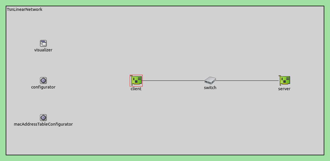
Two client devices each generate a traffic stream, one generating normal traffic with a steady data rate, the other misbehaving traffic with varying, sometimes excessive data rate. Both streams get forwarded to the server by the switch, while the combined traffic at times exceeds the capacity of the link between the switch and the server. We explore what happens with and without policing in the switch.
Traffic Configuration
The clients and the server are TsnDevice modules, and the switch is a TsnSwitch module. The links between them use 100Mbps EthernetLink channels.
Two distinct traffic patterns are generated. client1 produces misbehaving
traffic averaging 40Mbps using small 25-byte packets. The packet intervals
follow a dual-frequency sinusoidal pattern—two overlapping sine waves of
different frequencies—creating highly variable, bursty traffic. client2
generates steady normal traffic at 20Mbps using 500-byte packets at regular
intervals.
The misbehaving traffic uses small packets with high packet rates to provide finer temporal resolution in the data rate plots. However, this also means that the network data rate will be significantly higher than the 40Mbps application data rate due to protocol overhead. The combined traffic from both streams at times will exceed the 100Mbps channel capacity between the switch and the server, as we’ll see in the Results section.
The two streams are of the same traffic class. This is important because if they were in different classes, the problem could be solved by the traffic shaper. However, since they are the same class, the well-behaving and misbehaving streams are mixed in the shaper, so the problem must be solved through filtering.
The bridging layer identifies the outgoing packets by their UDP destination port.
# configure client applications
*.client*.numApps = 1
*.client*.app[*].typename = "UdpSourceApp"
*.client1.app[0].display-name = "misbehaving traffic"
*.client2.app[0].display-name = "normal traffic"
*.client*.app[0].io.destAddress = "server"
*.client1.app[0].io.destPort = 1000
*.client2.app[0].io.destPort = 1001
*.client1.app[0].io.displayStringTextFormat = "{numSent} misbehaving traffic"
*.client2.app[0].io.displayStringTextFormat = "{numSent} normal traffic"

# configure misbehaving traffic stream ~40Mbps
*.client1.app[0].source.packetLength = 25B
*.client1.app[0].source.productionInterval = 10us + replaceUnit(sin(dropUnit(simTime() * 10)), "ms") / 256 + replaceUnit(sin(dropUnit(simTime() * 125)), "ms") / 512


# configure normal traffic stream ~20Mbps
*.client2.app[0].source.packetLength = 500B
*.client2.app[0].source.productionInterval = 250us
Stream Identification and Classification
The clients identify and mark outgoing packets with VLAN IDs, while the switch decodes these markings to apply the appropriate policies:
# enable outgoing streams
*.client*.hasOutgoingStreams = true

# configure client stream identification
*.client*.bridging.streamIdentifier.identifier.mapping = [{stream: "misbehaving traffic", packetFilter: expr(udp.destPort == 1000)},
                                                          {stream: "normal traffic", packetFilter: expr(udp.destPort == 1001)}]

# configure client stream encoding
*.client*.bridging.streamCoder.encoder.mapping = [{stream: "misbehaving traffic", vlan: 0},
                                                  {stream: "normal traffic", vlan: 4}]

# disable forwarding IEEE 802.1Q C-Tag
*.switch.bridging.directionReverser.reverser.excludeEncapsulationProtocols = ["ieee8021qctag"]

# configure stream decoding
*.switch.bridging.streamCoder.decoder.mapping = [{vlan: 0, stream: "misbehaving traffic"},
                                                 {vlan: 4, stream: "normal traffic"}]
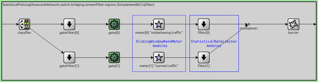
Per-Stream Filtering
The per-stream ingress filtering dispatches the different traffic classes to separate metering and filter paths:
*.switch.bridging.streamFilter.ingress.numStreams = 2
*.switch.bridging.streamFilter.ingress.hasDefaultPath = false
*.switch.bridging.streamFilter.ingress.classifier.mapping = {"misbehaving traffic": 0, "normal traffic": 1}
*.switch.bridging.streamFilter.ingress.meter[0].display-name = "misbehaving traffic"
*.switch.bridging.streamFilter.ingress.meter[1].display-name = "normal traffic"
Statistical Meter and Limiter Configuration
We use a SlidingWindowRateMeter combined with a StatisticalRateLimiter for both streams. The meter continuously measures the traffic rate over a sliding time window, while the limiter probabilistically drops packets when the measured rate exceeds the configured maximum.
Key parameters:
timeWindow: The duration over which traffic is measured (15ms for both streams)maxDatarate: The target rate limit (40Mbps for misbehaving traffic, 20Mbps for normal traffic)
As a rule of thumb, bursts significantly smaller than the time window are passed.
Note
Generally in policing, we want to allow some short bursts, and penalize sustained misbehaving traffic, while always staying below link capacity.
Here is the configuration:
*.switch*.bridging.streamFilter.ingress.meter[*].typename = "SlidingWindowRateMeter"
*.switch*.bridging.streamFilter.ingress.meter[*].timeWindow = 15ms
*.switch*.bridging.streamFilter.ingress.filter[*].typename = "StatisticalRateLimiter"
*.switch*.bridging.streamFilter.ingress.filter[0].maxDatarate = 40Mbps
*.switch*.bridging.streamFilter.ingress.filter[1].maxDatarate = 20Mbps
The following figure illustrates the per-stream filtering architecture, showing how traffic is classified, metered, and filtered inside the bridging layer of the switch:
Results
Without Policing
The first chart shows that one of the traffic streams is generating excessive, misbehaving traffic. Here is the application traffic generated by the clients:
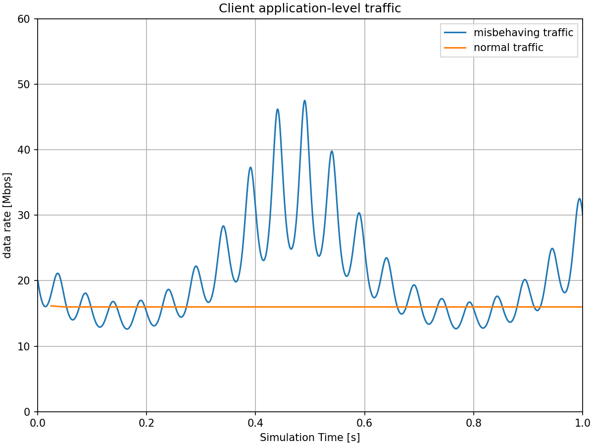
The combined application-level traffic averages approximately 60Mbps, but due to high protocol overhead of the misbehaving traffic—each 25-byte packet requires approximately 62 bytes of overhead (12B interframe gap, 8B Ethernet PHY preamble, 14B Ethernet MAC header, 20B IP header, 8B UDP header)—the misbehaving stream alone is enough to saturate a 100Mbps channel. The following chart shows the outgoing network-level traffic at client1 (misbehaving) and client2 (normal):
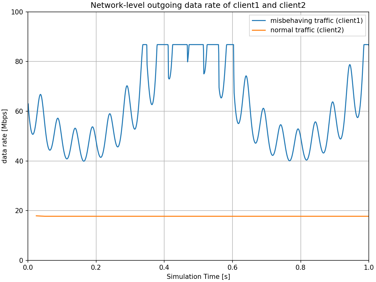
The misbehaving traffic stream is at times saturating the channel between client1 and the switch, which causes the visible clipping of the sinusoid traffic pattern at around 86 Mbps. This clipping occurs below the 100 Mbps channel capacity due to the large overhead from interframe gaps—with small 25-byte packets, a significant portion of the channel is consumed by the mandatory 12-byte interframe gap between packets.
The combined network traffic frequently exceeds the 100 Mbps channel capacity between the switch and the server. The next chart shows the traffic received at the server without policing:
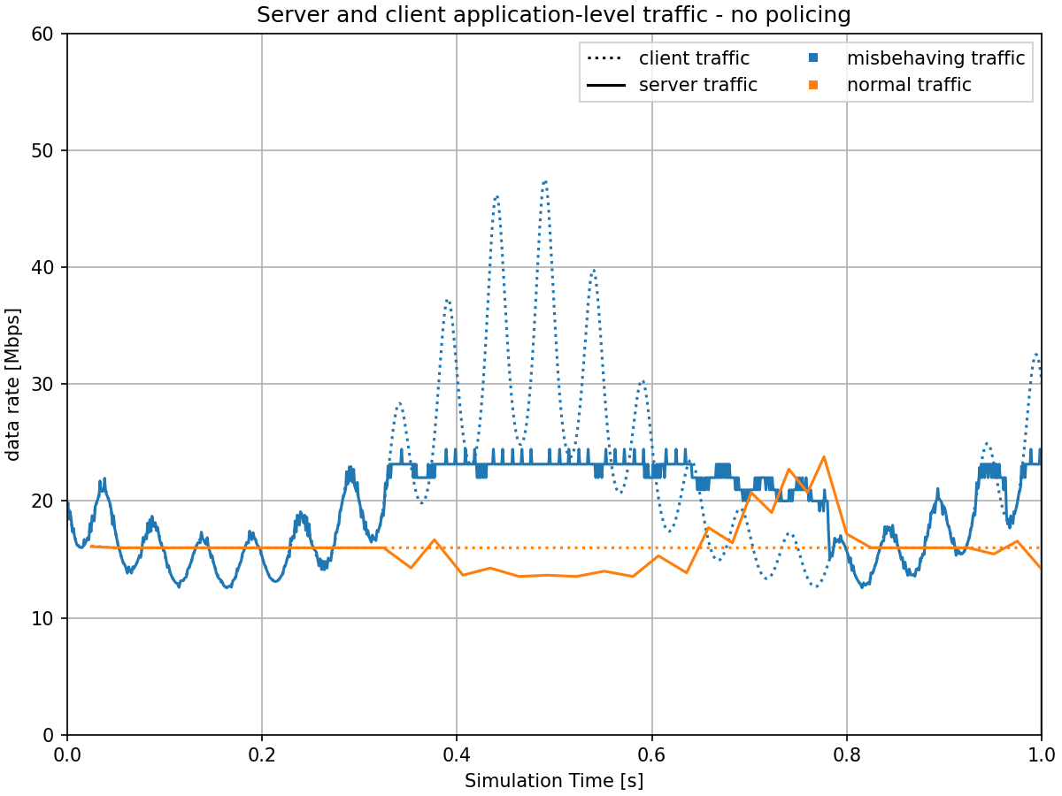
The misbehaving traffic competes with normal traffic for bandwidth, both slowing normal traffic down during congestion and occasionally speeding it up when the misbehaving traffic has lower rates.
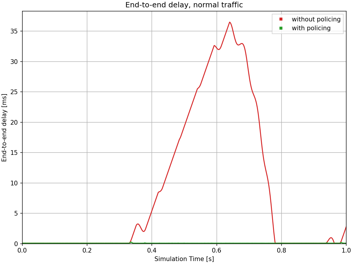
Here is the end-to-end delay of the normal stream:
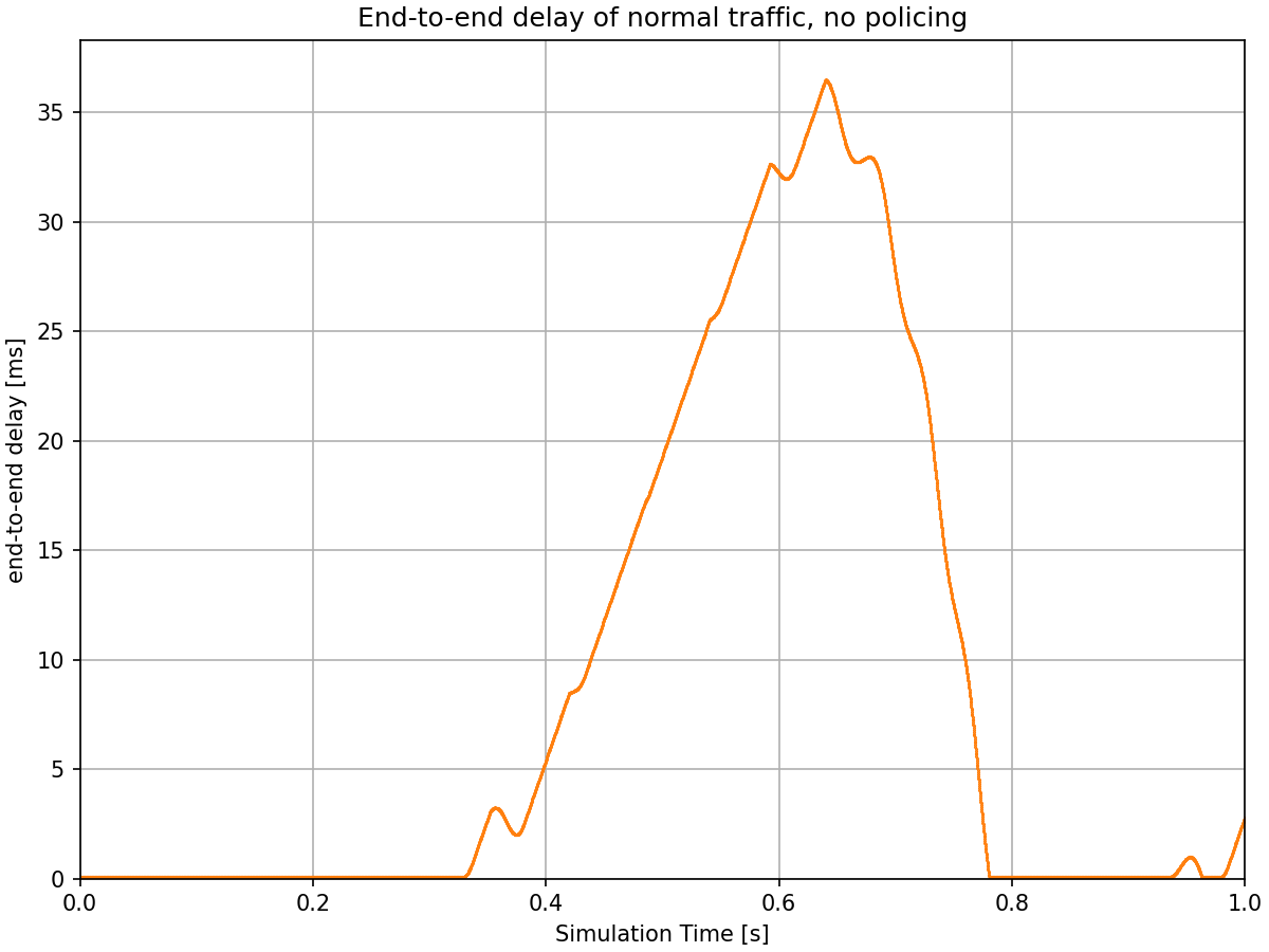
When the combined traffic exceeds the link capacity, packets must queue at the switch, leading to delays. Without policing, the normal traffic experiences significant delay spikes reaching up to almost 40 ms during periods when the misbehaving traffic is high. This demonstrates the problem: well-behaved traffic is disrupted by excessive traffic sources sharing the same network infrastructure.
With Policing
The next charts show how statistical policing solves this problem by limiting excessive, misbehaving traffic while protecting normal traffic.
Here is the application-level traffic at the server, comparing scenarios with and without policing:
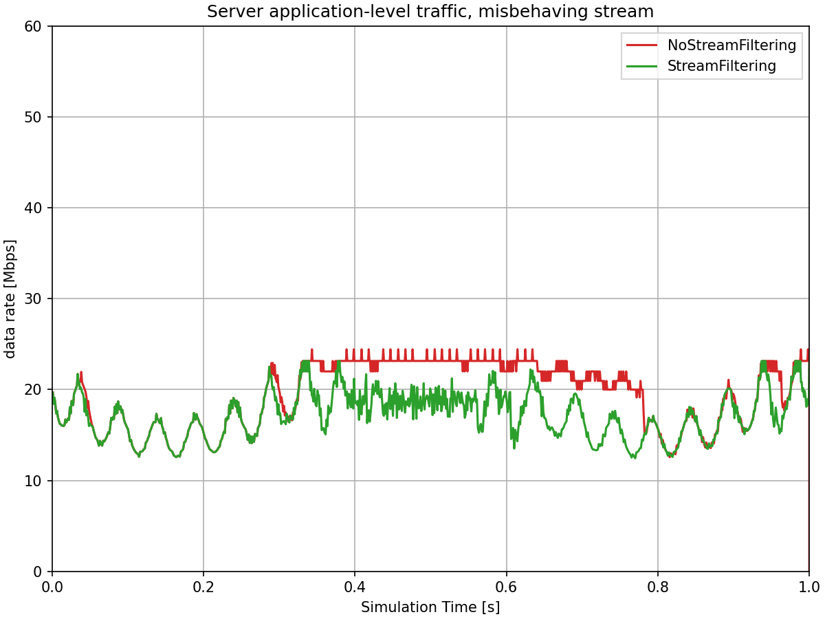
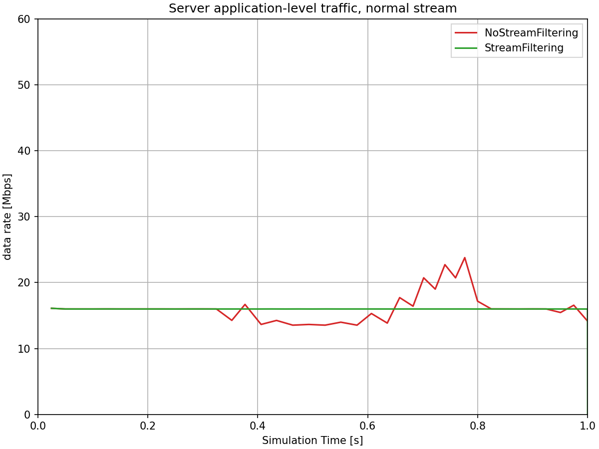
With statistical policing enabled in the switch’s ingress filter, the misbehaving traffic is now limited to approximately its configured maximum network-level data rate of 40 Mbps. Due to the small packets and large overhead, the application-level data rate in the server is lower, about 20Mbps. The statistical rate limiter probabilistically drops excess packets, enforcing the rate limit. The normal traffic continues to flow at its expected rate of 20 Mbps (network-level), unaffected by the excess traffic. The total traffic to the server stays well within the link capacity.
Note that the policed misbehaving traffic still shows fluctuation around the limit, rather than being strictly capped. This is characteristic of statistical policing: the sliding window rate meter measures traffic over a time window (15ms in this configuration), and the statistical rate limiter probabilistically drops packets based on the measured rate. This creates a gradual, probabilistic enforcement that allows some variation while maintaining the average rate at the configured limit. This is in contrast to token bucket policing, which creates sharper cutoffs when tokens are depleted.
The next chart shows the end-to-end delay of normal traffic, comparing scenarios with and without policing:
With policing enabled, the normal traffic experiences consistently low delays, typically around 0.1 ms, with not even a significant spike. The statistical policing mechanism has successfully protected the normal traffic from being disrupted by the misbehaving traffic stream. This demonstrates a key benefit of per-stream policing in TSN environments: ensuring predictable performance for well-behaved streams even when sharing network infrastructure with excessive traffic sources.
Additional Details
The following chart shows a zoomed view of the end-to-end delay of the normal stream, focusing on the time period when delays are low in both scenarios (with and without policing):
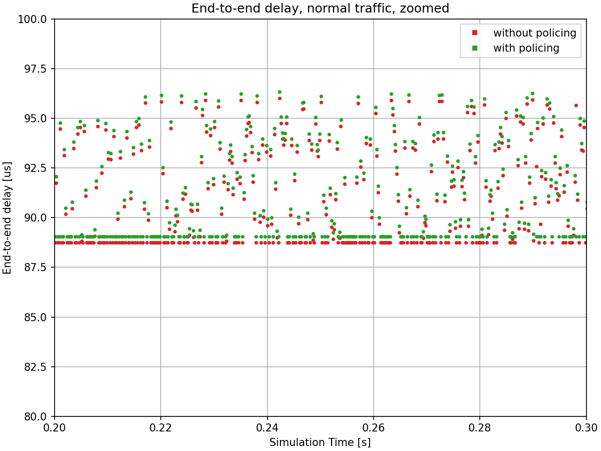
The delay variation occurs because both traffic streams are mixed in the switch’s output queue. When packets from both streams are queued simultaneously, a packet from one stream may need to wait for a packet from the other stream to complete transmission, introducing variable delays depending on remaining transmission duration.
Note the consistent offset between the two delay values: the scenario without policing shows slightly lower delays than the scenario with policing. This difference is due to the absence of VLAN tags (IEEE 802.1Q headers) in the non-policing configuration.
The remaining charts provide insight into how the statistical policing mechanism operates internally.
Let’s see the incoming, outgoing, and dropped data rates in the misbehaving traffic’s filter. Additionally, the data rate measured by the meter is also displayed:
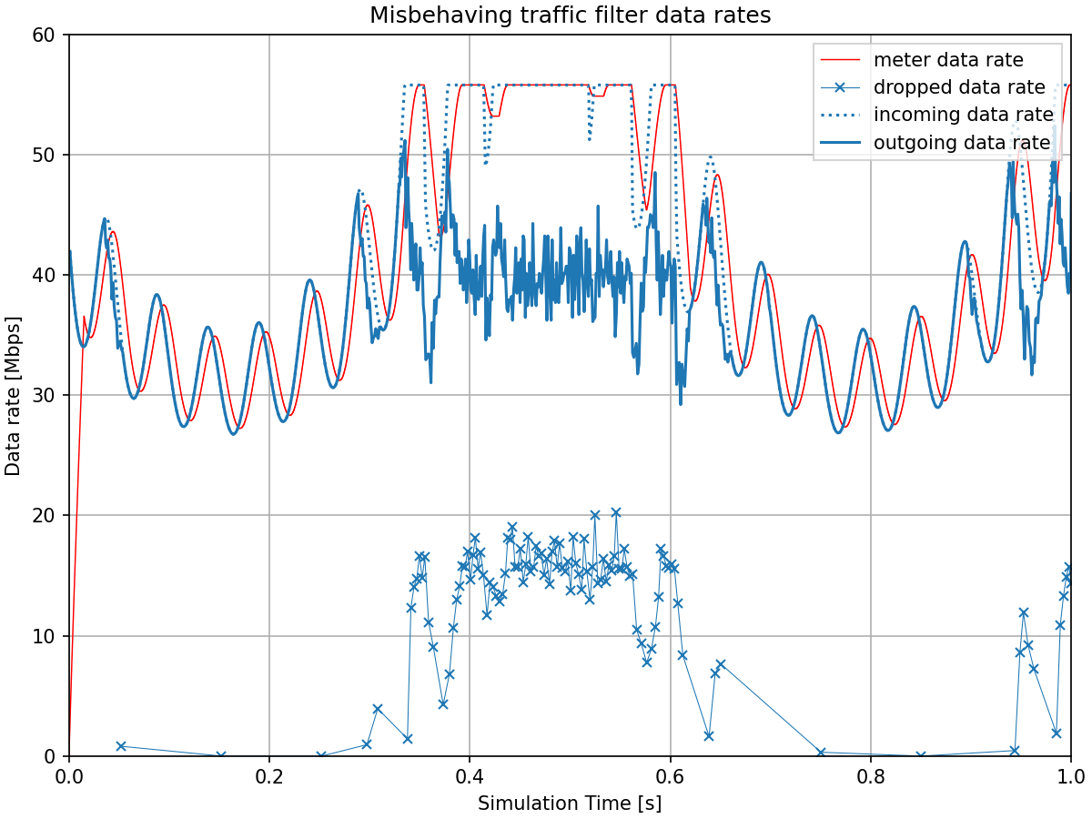
The traffic filter starts dropping packets when the measured data rate line (from the sliding window meter) exceeds 40 Mbps. The measured data rate shows a lag behind the incoming traffic. This delay occurs because the meter must accumulate 15ms worth of packet data before it can produce a measurement. A shorter time window would reduce this measurement lag but would also make the meter more reactive to short bursts.
This time window parameter represents a trade-off between two factors: a longer window allows bursts with shorter intervals to pass through but introduces more measurement lag, while a shorter window reduces the lag but filters out even brief bursts more aggressively.
In this chart, we can observe both effects: the 15ms window allows the initial short, high-frequency bursts to pass through largely intact (visible at the start of the chart), while the later sustained high traffic is limited by the filter, with the outgoing rate stabilizing around the configured 40 Mbps limit.
Now let’s see the same for the normal traffic’s filter:
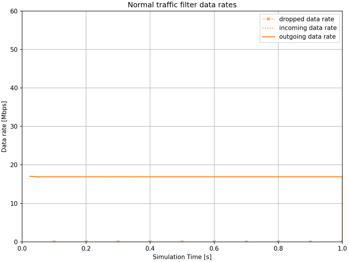
The normal traffic filter shows that all packets pass through with no drops, since the traffic operates well within its configured 20 Mbps limit.
Sources: omnetpp.ini
Try It Yourself
If you already have INET and OMNeT++ installed, start the IDE by typing
omnetpp, import the INET project into the IDE, then navigate to the
inet/showcases/tsn/streamfiltering/statistical folder in the Project Explorer. There, you can view
and edit the showcase files, run simulations, and analyze results.
Otherwise, there is an easy way to install INET and OMNeT++ using opp_env, and run the simulation interactively.
Ensure that opp_env is installed on your system, then execute:
$ opp_env run inet-4.6 --init -w inet-workspace --install --build-modes=release --chdir \
   -c 'cd inet-4.6.*/showcases/tsn/streamfiltering/statistical && inet'
This command creates an inet-workspace directory, installs the appropriate
versions of INET and OMNeT++ within it, and launches the inet command in the
showcase directory for interactive simulation.
Alternatively, for a more hands-on experience, you can first set up the workspace and then open an interactive shell:
$ opp_env install --init -w inet-workspace --build-modes=release inet-4.6
$ cd inet-workspace
$ opp_env shell
Inside the shell, start the IDE by typing omnetpp, import the INET project,
then start exploring.
Discussion
Use this page in the GitHub issue tracker for commenting on this showcase.