Clock Drift
Goals
In the real world, there is no globally agreed-upon time, but each node uses its own physical clock to keep track of time. Due to finite clock accuracy, the time of clocks in various nodes of the network may diverge over time. Clock drift refers to this gradual deviation. To address the issue of clock drift, time synchronization mechanisms can be used to periodically adjust the clocks of network devices to ensure that they remain adequately in sync with each other.
The operation of applications and protocols across the network is often very sensitive to the accuracy of this local time. Time synchronization is important in TSN, for example, as accurate time-keeping is crucial in these networks.
In this showcase, we will demonstrate how to introduce local clocks in network nodes and how to configure clock drift for these clocks. We will also show how to use time synchronization mechanisms to reduce time differences between the clocks of different devices.
4.6Simulating Clock Drift and Time Synchronization
By default, modules such as network nodes and interfaces in INET don’t have local time but use the simulation time as a global time. To simulate network nodes with local time, and effects such as clock drift and its mitigation (time synchronization), network nodes need to have clock submodules. To keep time, most clock modules use oscillator submodules. The oscillators produce ticks periodically, and the clock modules count the ticks. Clock drift is caused by inaccurate oscillators. INET provides various oscillator models, so by combining clock and oscillator models, we can simulate constant and random clock drift rates. To model time synchronization, the time of clocks can be set by synchronizer modules.
Several clock models are available:
OscillatorBasedClock: Has an oscillator submodule; keeps time by counting the oscillator’s ticks. Depending on the oscillator submodule, can model constant and random clock drift rate
SettableClock: Same as the oscillator-based clock but the time can be set from C++ or a scenario manager script
IdealClock: The clock’s time is the same as the simulation time; for testing purposes
The following oscillator models are available:
IdealOscillator: generates ticks periodically with a constant tick length
ConstantDriftOscillator: generates ticks periodically with a constant drift rate in generation speed; for modeling constant rate clock drift
RandomDriftOscillator: the oscillator changes drift rate over time; for modeling random clock drift
Synchronizers are implemented as application-layer modules. For clock synchronization, the synchronizer modules need to set the time of clocks, thus only the SettableClock supports synchronization. The following synchronizer modules are available:
SimpleClockSynchronizer: Uses an out-of-band mechanism to synchronize clocks, instead of a real clock synchronization protocol. Useful for simulations where the details of time synchronization are not important.
Gptp: Uses the General Precision Time Protocol to synchronize clocks.
The SimpleClockSynchronizer module periodically synchronizes a slave clock to a master clock. The synchronization interval can be configured with a parameter. Also, in order to model real-life synchronization protocols, which are somewhat inaccurate by nature, the accuracy can be specified (see the NED documentation of the module for more details).
The General Precision Time Protocol (gPTP, or IEEE 802.1 AS) can synchronize
clocks in an Ethernet network with a high clock accuracy required by TSN
protocols. It is implemented in INET by the Gptp module. Several network
node types, such as EthernetSwitch have optional gPTP modules, activated
by the hasGptp boolean parameter. It can also be inserted into hosts as
one of the applications. Gptp is demonstrated in the last example of this
showcase. For more details about Gptp, check out the
Using gPTP showcase or the
module’s NED documentation.
When synchronization happens, both synchronizers update the current time of the clocks. Additionally, they update the drift rate of the clocks as well, by setting the oscillator compensation. SimpleClockSynchronizer reads the actual clock drift rate with an out-of-band mechanism, and sets the oscillator compensation accordingly. With Gptp, the oscillator compensation is set based on the last two time synchronization events.
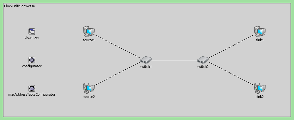
The Model and Results
The showcase contains several example simulations. All simulations use the following network:
The example configurations are the following:
NoClockDrift: Network nodes don’t have clocks, they are synchronized by simulation timeConstantClockDrift: Network nodes have clocks with constant clock drift rate, and the clocks diverge over timeConstantClockDriftOutOfBandSync: Clocks have a constant drift rate, and they are synchronized by an out-of-band synchronization method (without a real protocol)RandomClockDrift: Clocks have a periodically changing random clock drift rateRandomClockDriftOutOfBandSync: Clocks have a periodically changing random clock drift rate, and they are synchronized by an out-of-band synchronization method (without a real protocol)RandomClockDriftGptpSync: Clocks have random a periodically changing random clock drift rate, and they are synchronized by gPTP
In the General configuration, source1 is configured to send UDP packets to sink1, and source2 to sink2.
Note
To demonstrate the effects of drifting clocks on the network traffic, we configure the Ethernet MAC layer in switch1 to alternate between forwarding frames from source1 and source2 every 10 us, by using a TSN gating mechanism in switch1. This does not affect the simulation results in the next few sections but becomes important in the Effects of Clock Drift on End-to-end Delay section. More details about this part of the configuration are provided there.
In the next few sections, we present the above examples. In the simulations
featuring constant clock drift, switch1 always has the same clock drift
rate. In the random drift configurations, the drift rate is specified with the
same distribution, but the actual drift rates can differ between configurations.
In the configurations also featuring clock synchronization, the hosts are
synchronized to the time of switch1. We plot the time difference of clocks
and simulation time to see how the clocks diverge from the simulation time and
each other.
Example: No Clock Drift
In this configuration, network nodes don’t have clocks. Applications and gate schedules are synchronized by simulation time. (End-to-end delays in the other three cases will be compared to this baseline configuration.)
There are no clocks, so the configuration is empty:
[Config NoClockDrift]
description = "Without clocks, network nodes are synchronized by simulation time"
Example: Constant Clock Drift Rate
In this configuration, all network nodes have a clock with a constant drift rate. Clocks drift away from each other over time.
Here is the configuration:
[Config ConstantClockDrift]
description = "Clocks with constant drift rate diverge over time"

*.*.clock.oscillator.nominalTickLength = 10ns

*.source*.clock.typename = "OscillatorBasedClock"
*.source*.clock.oscillator.typename = "ConstantDriftOscillator"
*.source1.clock.oscillator.driftRate = 500ppm
*.source2.clock.oscillator.driftRate = -400ppm
*.source*.app[0].source.clockModule = "^.^.clock"

*.switch1.clock.typename = "OscillatorBasedClock"
*.switch1.clock.oscillator.typename = "ConstantDriftOscillator"
*.switch1.clock.oscillator.driftRate = 300ppm
*.switch1.eth[0].macLayer.queue.gate[*].clockModule = "^.^.^.^.clock"
We configure the network nodes to have OscillatorBasedClock modules, with
a ConstantDriftOscillator. We also set the drift rate of the oscillators.
By setting different drift rates for the different clocks, we can control how
they diverge over time. Note that the drift rate is defined as compared to
simulation time. Also, we need to explicitly tell the relevant modules (here,
the UDP apps and switch1’s queue) to use the clock module in the host,
otherwise, they would use the global simulation time by default.
We set the nominalTickLength parameter of all oscillators to 10ns, which is a typical value for
real-world clocks. To be able to represent 1 PPM clock drift, we set fs simulation time accuracy (10ns / 10^6 = 10fs).
Here are the drifts (time differences) over time:
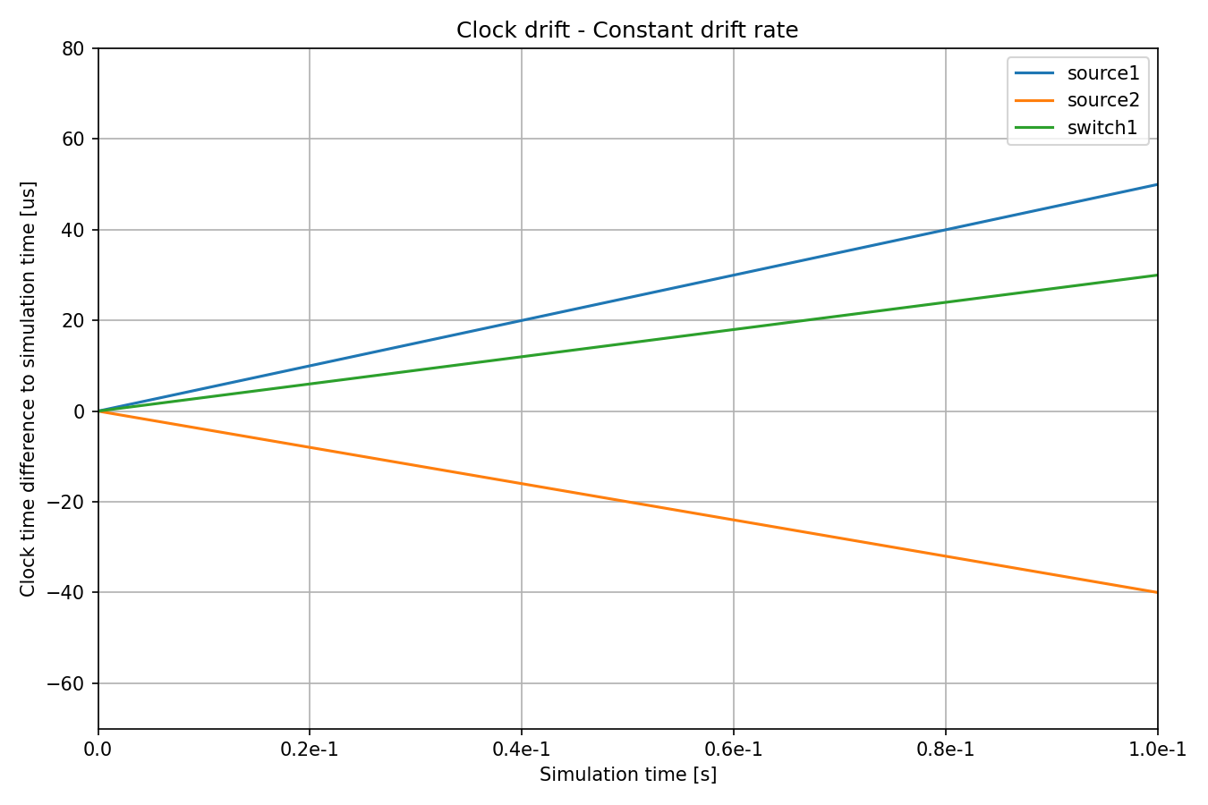
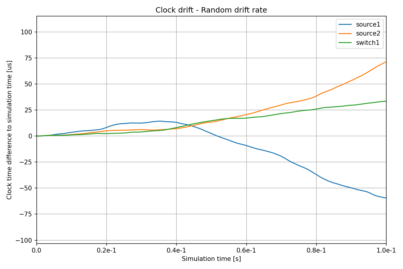
The three clocks have different drift rates. The magnitude and direction of
drift of source1 and source2 compared to switch1 are different as
well, i.e. source1’s clock is early and source2’s clock is late compared
to switch1’s.
Note
A clock time difference to the simulation time chart can be easily produced by plotting the timeChanged:vector statistic and applying a linear trend operation with -1 as the argument.
Example: Out-of-Band Synchronization of Clocks, Constant Drift
In this configuration, the network node clocks have the same constant drift rate as in the previous configuration, but they are periodically synchronized by an out-of-band mechanism (C++ function call).
The out-of-band synchronization settings are defined in a base configuration, OutOfBandSyncBase, that we can extend:
[Config OutOfBandSyncBase]
description = "Base config for out-of-band synchronization"
abstract = true

*.source*.clock.typename = "SettableClock"
*.source*.clock.defaultOverdueClockEventHandlingMode = "execute"

*.source*.numApps = 2
*.source*.app[1].typename = "SimpleClockSynchronizer"
*.source*.app[1].masterClockModule = "^.^.switch1.clock"
*.source*.app[1].slaveClockModule = "^.clock"
*.source*.app[1].synchronizationInterval = 500us
*.source*.app[1].synchronizationClockTimeError = uniform(-10ns, 10ns)
Since we want to use clock synchronization, we need to be able to set the
clocks, so network nodes have SettableClock modules. The
defaultOverdueClockEventHandlingMode = "execute" setting means that when
setting the clock forward, events that become overdue are done immediately. We
use the SimpleClockSynchronizer for out-of-band synchronization.
Synchronizer modules are implemented as applications, so we add one to each
source host in an application slot. We set the synchronizer modules to sync time
to the clock of switch1. We specify a small random clock time error for the
synchronization, thus the clock times will not be synchronized perfectly.
For the constant clock drift rate, this configuration extends
ConstantClockDrift. For the synchronization, it extends
OutOfBandSyncBase as well. Otherwise, the configuration is empty:
[Config ConstantClockDriftOutOfBandSync]
description = "Clocks are periodically synchronized out-of-band, without a real protocol. Clocks use constant drift oscillators."
extends = OutOfBandSyncBase, ConstantClockDrift
Let’s see the time differences:
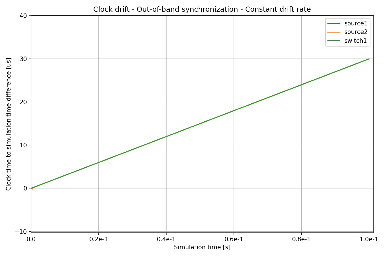
The clock of switch1 has a constant drift rate compared to simulation time.
Since the clock drift rate in all clocks is constant, the drift rate differences
are compensated for after the first synchronization event by setting the
oscillator compensation in the synchronized clocks. After that, all
clocks have the same drift rate as the clock of switch1. Let’s zoom in on
the beginning of the above chart:
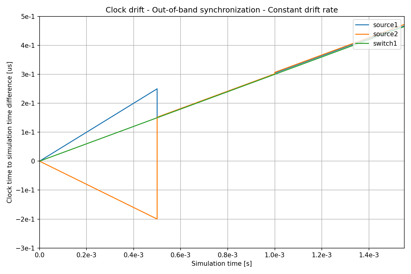
At the beginning of the simulation, the clocks have a different drift rate, until the drift rate is compensated for at the first synchronization event. The drift rate is compensated for with no error, but time is synchronized with a small random error we configured (note the small distance between the lines after synchronization, which randomly varies at each sync event).
Example: Random Clock Drift Rate
In this configuration, clocks utilize the RandomDriftOscillator module, which periodically changes the drift rate through a random walk process. The magnitude of drift rate change is specified as a distinct distribution for each oscillator. Additionally, the interval of drift rate change is set to be constant. Here is the configuration:
[Config RandomClockDrift]
description = "Clocks with random drift rate"

*.*.clock.oscillator.nominalTickLength = 10ns

*.source*.clock.typename = "OscillatorBasedClock"
*.source*.clock.oscillator.typename = "RandomDriftOscillator"
*.source1.clock.oscillator.driftRateChange = uniform(-125ppm, 125ppm)
*.source2.clock.oscillator.driftRateChange = uniform(-100ppm, 100ppm)
*.source1.clock.oscillator.changeInterval = 0.1ms
*.source2.clock.oscillator.changeInterval = 0.1ms
*.source*.app[0].source.clockModule = "^.^.clock"

*.switch1.clock.typename = "OscillatorBasedClock"
*.switch1.clock.oscillator.typename = "RandomDriftOscillator"
*.switch1.clock.oscillator.driftRateChange = uniform(-75ppm, 75ppm)
*.switch1.clock.oscillator.changeInterval = 0.1ms
*.switch1.eth[0].macLayer.queue.gate[*].clockModule = "^.^.^.^.clock"
Note
In reality, the typical drift rate change is very small, 1 PPM/s. We use higher values so that the changes are more visible.
The following chart displays how the clocks diverge over time:
Example: Out-of-Band Synchronization of Clocks, Random Drift
This configuration extends the previous one with a periodic out-of-band
synchronization mechanism (using cross-network node C++ function calls), defined
in the OutOfBandSyncBase configuration:
[Config RandomClockDriftOutOfBandSync]
description = "Clocks are periodically synchronized out-of-band, without a real protocol. Clocks use random drift oscillators."
extends = OutOfBandSyncBase, RandomClockDrift
As with the constant drift rate + out-of-band synchronization case, we specify a small random clock time synchronization error, but no drift rate synchronization error.
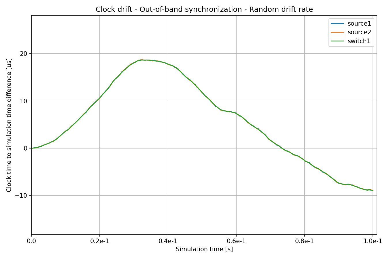
The clock of switch1 keeps drifting, but the clocks of the sources are
synchronized to it. Here is the same chart, but zoomed in:
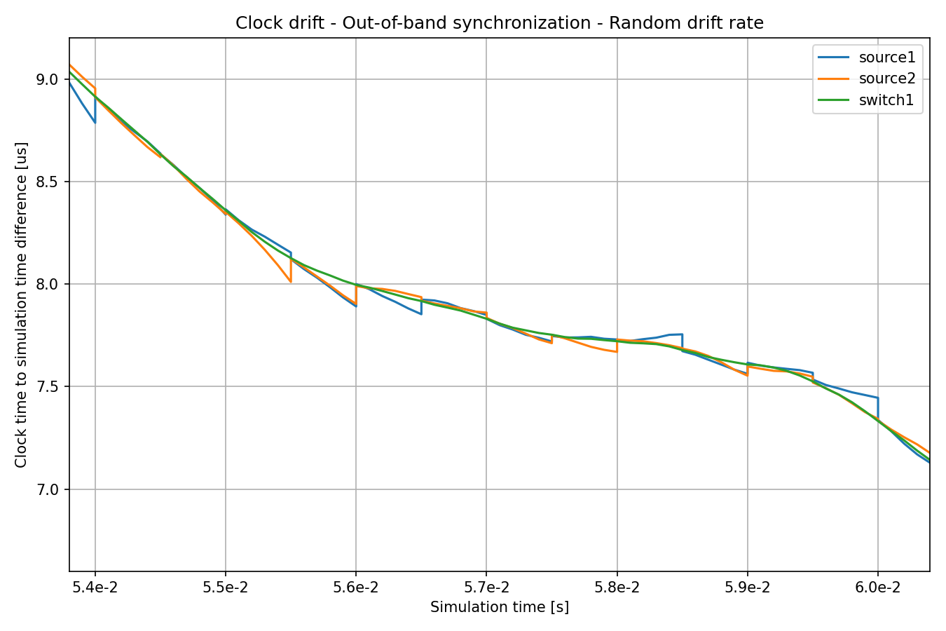
The rate of clock drift is perfectly synchronized, so the lines for the sources
are tangential to switch1’s at the synchronization points. However, the
clocks drift between synchronization events, so the divergence increases until
synchronized again.
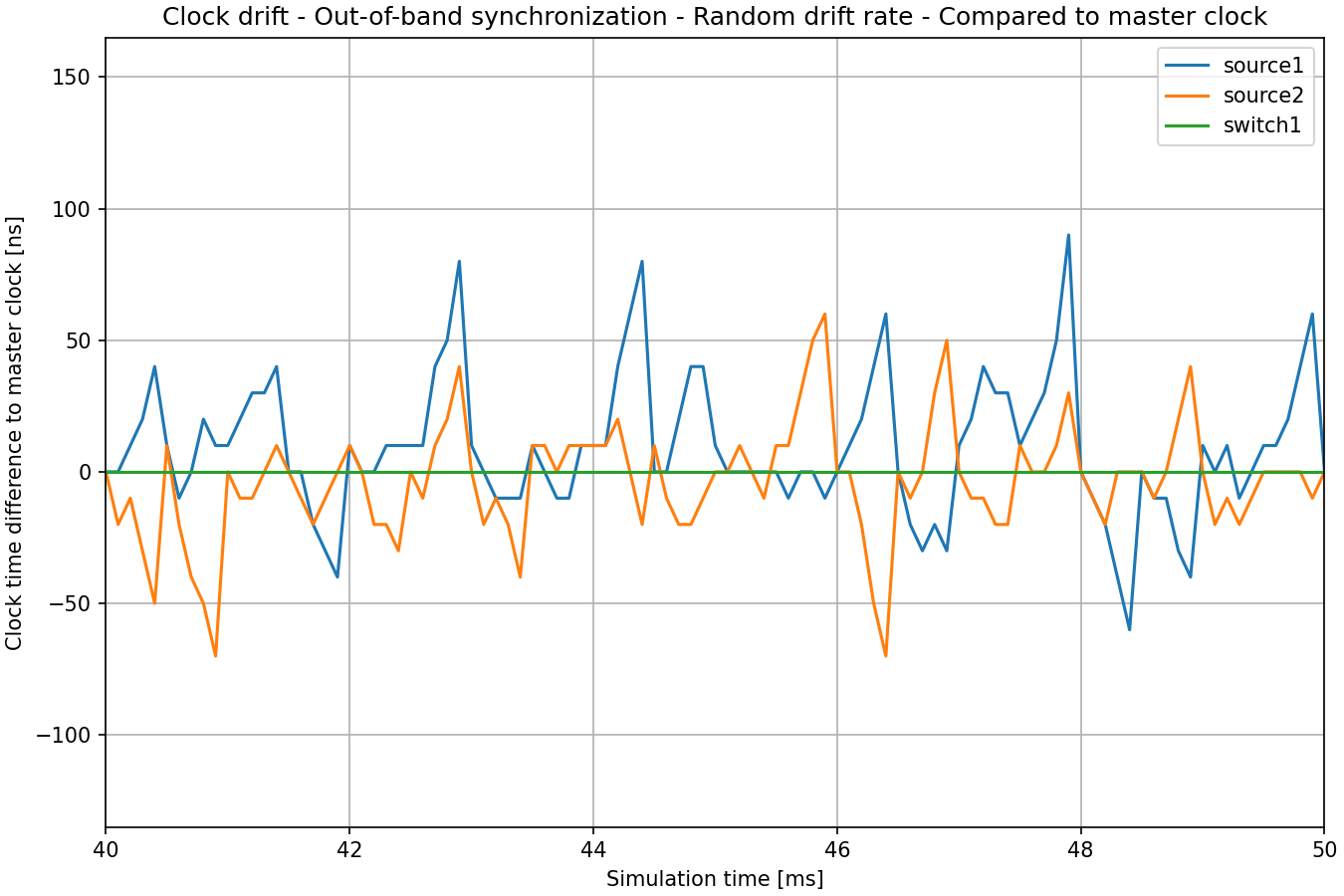
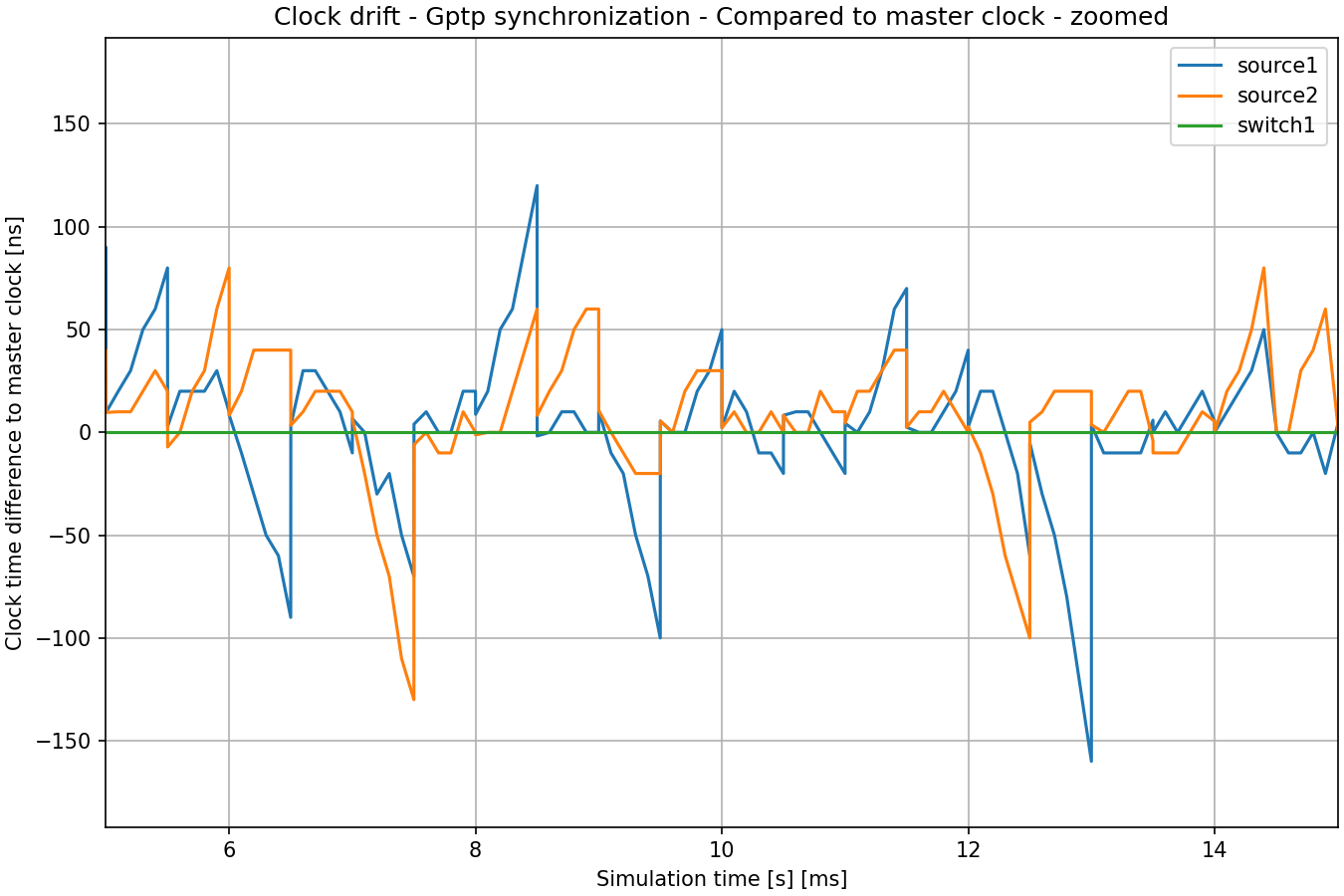
The following chart shows the clock time difference to the master clock (switch1). This is the
most important statistic of time synchronization in TSN.
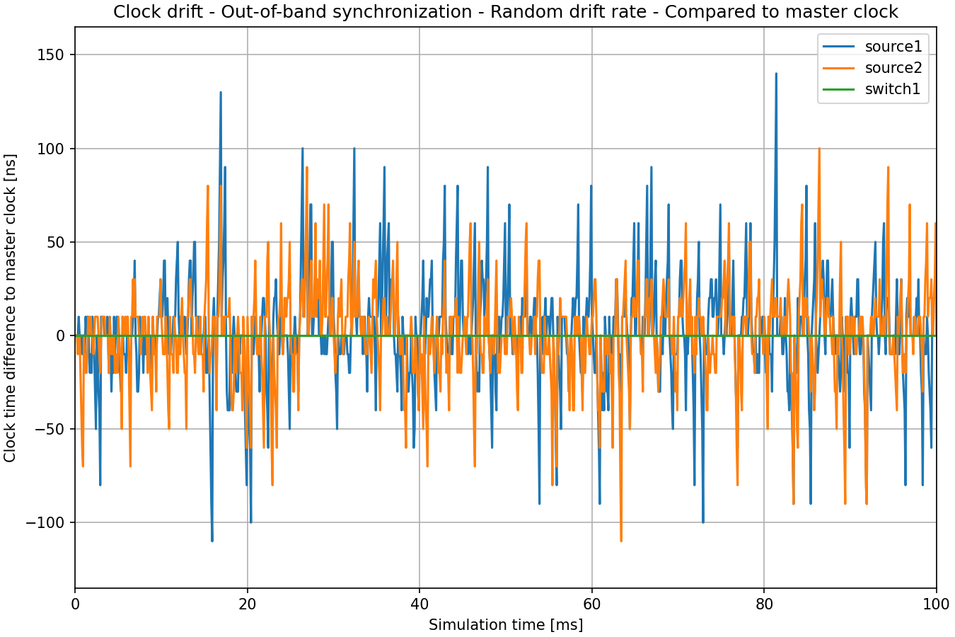
Here is the same chart zoomed in:
Example: Synchronizing Clocks Using gPTP
In this configuration, the clocks in network nodes have the same drift rates as in the previous two configurations, but they are periodically synchronized to a master clock using the Generic Precision Time Protocol (gPTP). The protocol measures the delay of individual links and disseminates the clock time of the master clock on the network through a spanning tree.
Here is the configuration:
[Config RandomClockDriftGptpSync]
description = "Clocks are periodically synchronized using gPTP"
extends = RandomClockDrift

*.switch*.hasGptp = true

*.switch*.gptp.syncInterval = 500us
*.switch*.gptp.pdelayInterval = 1ms
*.switch*.gptp.pdelayInitialOffset = 0ms

*.switch*.clock.typename = "SettableClock"

*.switch1.gptp.gptpNodeType = "MASTER_NODE"
*.switch1.gptp.masterPorts = ["eth0", "eth1", "eth2"]  # eth*

*.switch2.gptp.gptpNodeType = "SLAVE_NODE"
*.switch2.gptp.slavePort = "eth0"

*.source*.clock.typename = "SettableClock"

*.source*.numApps = 2
*.source*.app[1].typename = "Gptp"
*.source*.app[1].gptpNodeType = "SLAVE_NODE"
*.source*.app[1].slavePort = "eth0"
*.source*.app[1].syncInterval = 500us
*.source*.app[1].pdelayInterval = 1ms
Note
Gptp requires transmission start and reception start timestamps, which are not provided by the default physical layer. Thus, we use StreamingTransmitter and DestreamingReceiver.
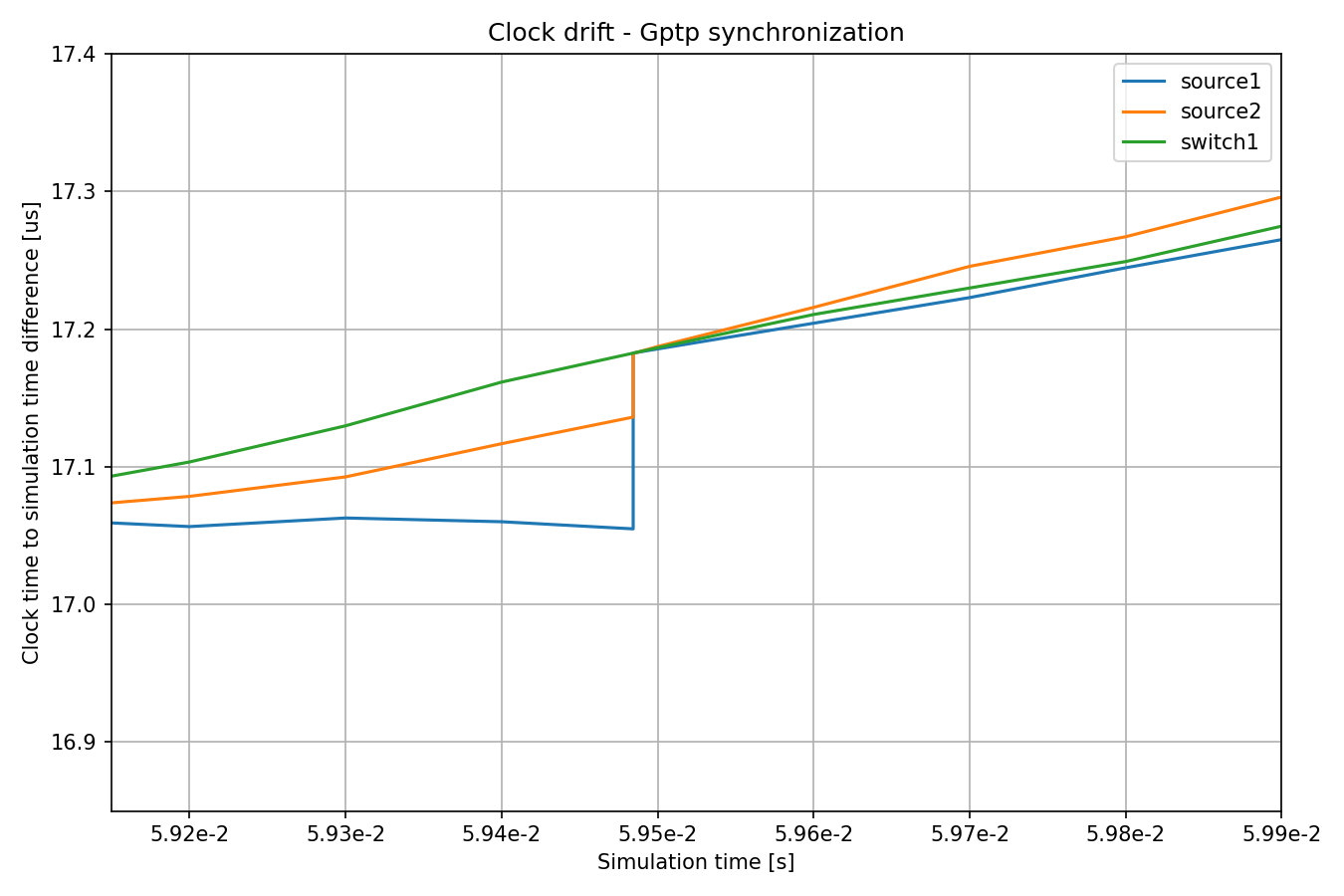
Here are the time differences:
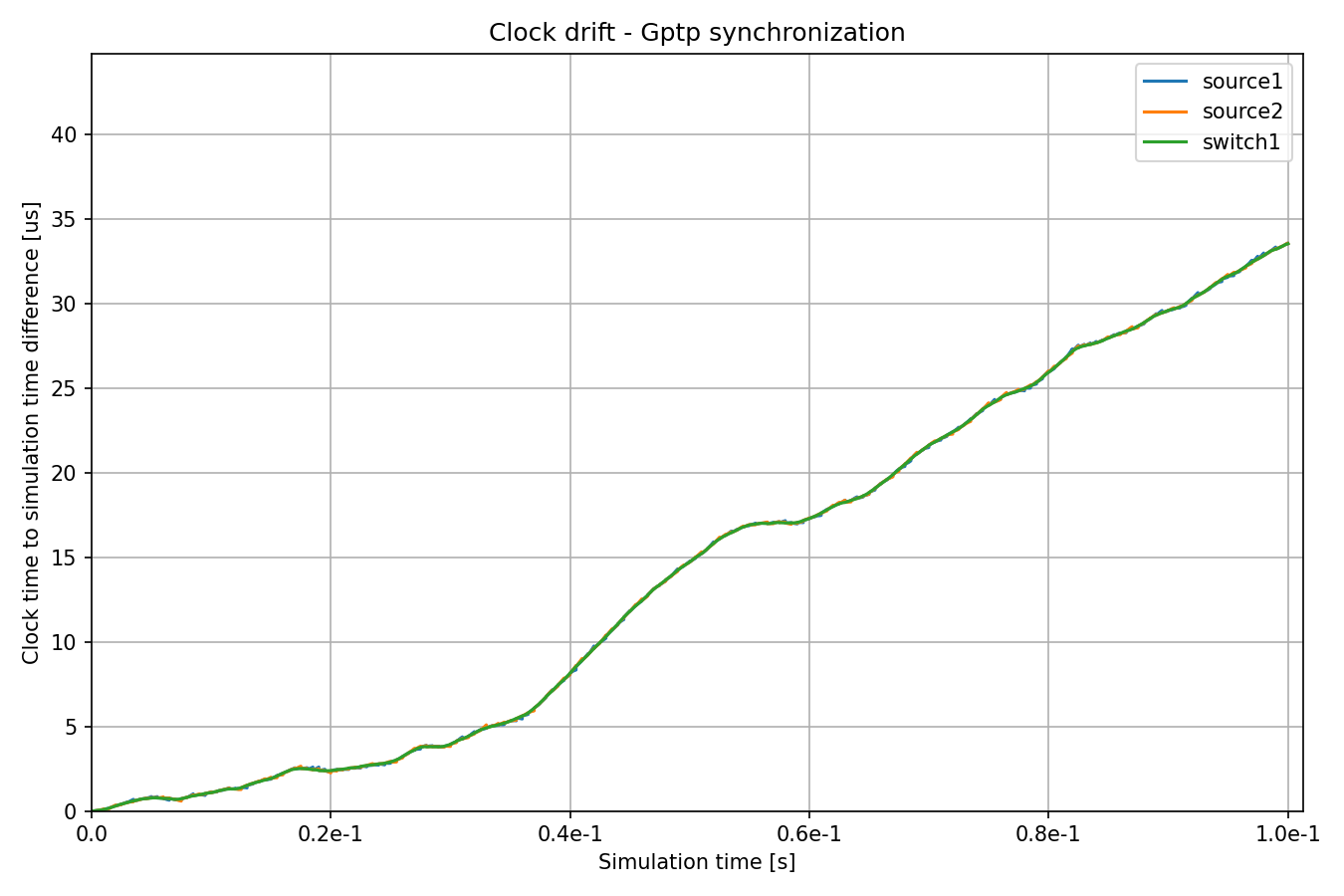
The clock of switch1 has a periodically changing random drift rate, and the
other clocks periodically synchronize to switch1.
Here is the above chart zoomed in:
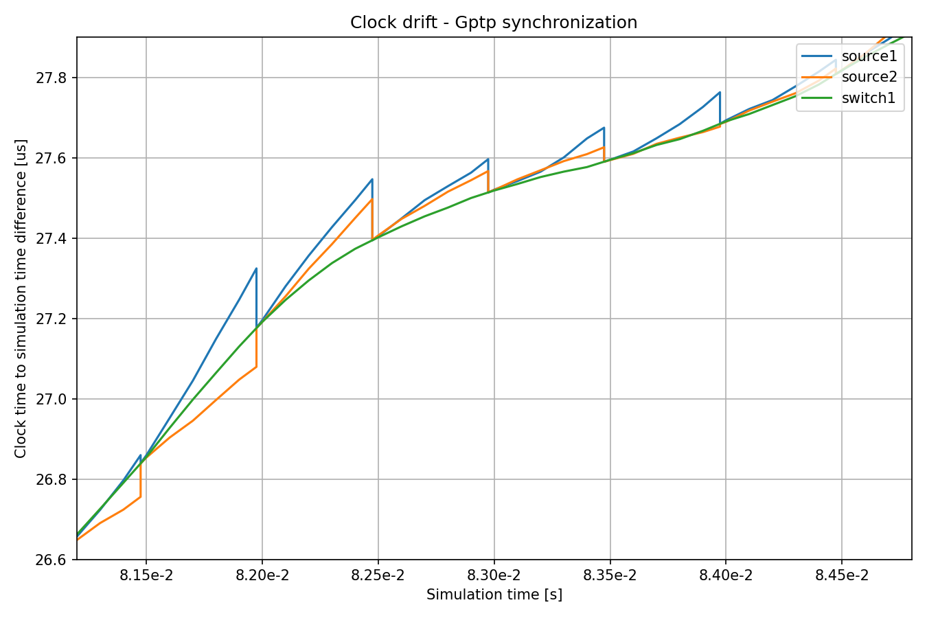
The drift rate difference, calculated from the previous two synchronization events, is used to set the oscillator compensation.
The following chart shows the clock time difference to the master clock (switch1):
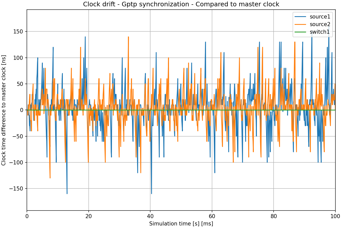
Here is the same chart zoomed in:
Accuracy of Synchronization
The precision of time synchronization can be visualized by zooming in on the above clock time charts. We can examine the moment when the times of the source hosts change. The distance of the new time from the reference shows the precision in time synchronization:
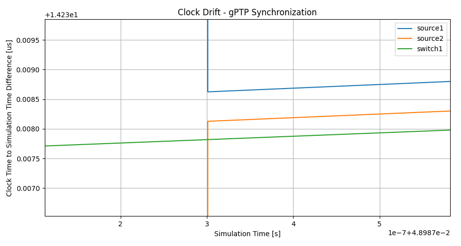
When the clocks are synchronized, the drift rate differences are also compensated for by setting the oscillator compensation in clocks. We can observe this on the following zoomed-in image:
Synchronization makes the lines more parallel, i.e. drift rates more closely match each other. Also, note that the drift rate sometimes changes between synchronization events due to the random walk process.
We configured a time synchronization error with a random distribution for the SimpleClockSynchronizer, but no drift rate compensation errors. In the case of gPTP, the accuracy is not settable but an emergent property of the protocol’s operation. Also, gPTP synchronization inherently has some drift rate compensation errors.
Note
When configuring the SimpleClockSynchronizer with a
synchronizationClockTimeErrorof 0, the synchronized time perfectly matches the reference.When configuring the SimpleClockSynchronizer with a
synchronizationOscillatorCompensationErrorof 0, the compensated clock drift rate perfectly matches the reference. Otherwise, the error can be specified in PPM.When using any of the synchronization methods, the clock time difference between the clocks is very small, in the order of microseconds.
Effects of Clock Drift on End-to-end Delay
This section aims to demonstrate that clock drift can have profound effects on the operation of the network. We take a look at the end-to-end delay in the four examples to show this effect.
To this end, in all simulations, the Ethernet MAC layer in switch1 is
configured to alternate forwarding packets from source1 and source2
every 10 us; note that the UDP applications are sending packets every 20 us,
with packets from source2 offset by 10 us compared to source1. Thus
packets from both sources have a send window in switch1, and the sources
generate and send packets to switch1 in sync with that send window (they are
only in sync if the clocks in the nodes are in sync, as we’ll see later).
Here is how we configure this. We configure the EthernetMacLayer in switch1
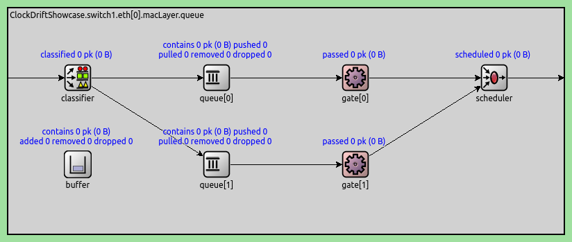
to contain a GatingPriorityQueue, with two inner queues:
*.switch1.eth[0].macLayer.queue.typename = "GatingPriorityQueue"
*.switch1.eth[0].macLayer.queue.numQueues = 2
The inner queues in the GatingPriorityQueue each have their own gate. The gates connect to a PriorityScheduler, so the gating priority queue prioritizes packets from the first inner queue. Here is a gating priority queue with two inner queues:
In our case, we configure the classifier (set to ContentBasedClassifier) to send
packets from source1 to the first queue and those from source2 to the
second, thus the gating priority queue prioritizes packets from source1. The
gates are configured to open and close every 10us, with the second gate offset
by a 10us period (so they alternate being open). Furthermore, we align the gate
schedules with the traffic generation by offsetting both gate schedules with
3.118us, the time it takes for a packet to be transmitted from a source to
switch1. Here is the rest of the gating priority queue configuration:
*.switch1.eth[0].macLayer.queue.classifier.typename = "ContentBasedClassifier"
*.switch1.eth[0].macLayer.queue.classifier.packetFilters = ["source1*", "source2*"]
*.switch1.eth[0].macLayer.queue.queue[*].typename = "DropTailQueue"
*.switch1.eth[0].macLayer.queue.gate[*].initiallyOpen = false
*.switch1.eth[0].macLayer.queue.gate[*].durations = [10us, 10us]
*.switch1.eth[0].macLayer.queue.gate[0].offset = 3.118us
*.switch1.eth[0].macLayer.queue.gate[1].offset = 13.118us
As mentioned before, the traffic applications in the sources generate packets
every 20us, with source2 offset from source1 by 10us:
# source applications
*.source*.numApps = 1
*.source*.app[*].typename = "UdpSourceApp"
*.source*.app[0].source.packetLength = 800B
*.source*.app[0].source.productionInterval = 20us
*.source*.app[0].io.destPort = 1000

*.source1.app[0].io.destAddress = "sink1"
*.source1.app[0].source.packetNameFormat = "source1-%c"

*.source2.app[0].io.destAddress = "sink2"
*.source2.app[0].source.initialProductionOffset = 10us
*.source2.app[0].source.packetNameFormat = "source2-%c"

# sink applications
*.sink*.numApps = 1
*.sink*.app[*].typename = "UdpSinkApp"
*.sink*.app[0].io.localPort = 1000
Note that only one data packet fits into the send window. However, gPTP packets are small and are sent in the same send windows as data packets.
We measure the end-to-end delay of packets from the source applications to the corresponding sink applications. Let’s examine the results below.
First, we take a look at the out-of-band synchronization cases. In the case of no clock drift, packet generation is perfectly aligned in time with gate schedules, thus packets always find the gates open. End-to-end delay is constant, as it stems from transmission time only (no queuing delay due to closed gates). This delay value is displayed on the charts as a baseline:
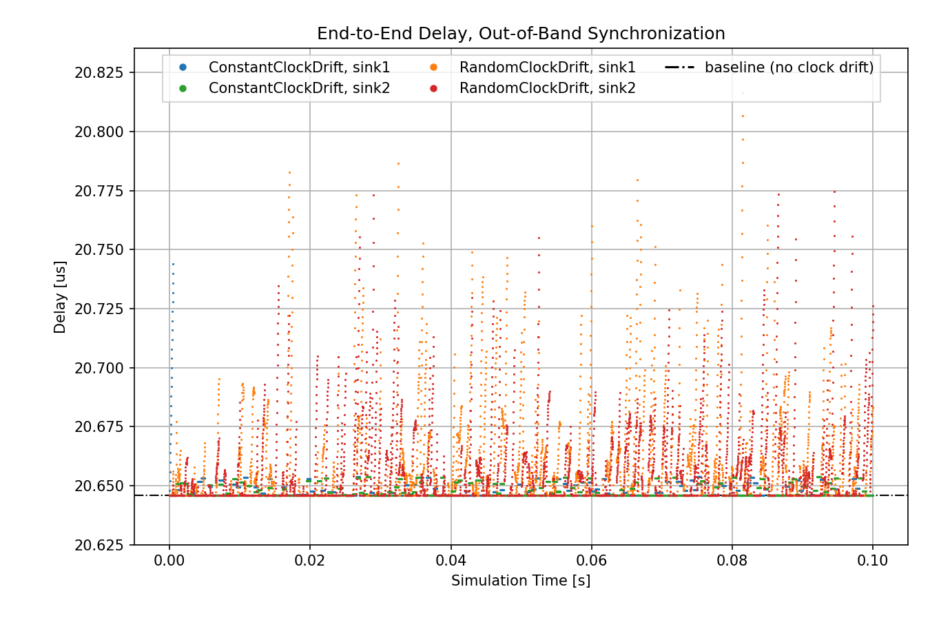
At the beginning of the simulation, the delay for constant drift/sink1 is large because the drift rate difference between the clocks is not yet synchronized. After that, however, its delay is lower and bounded. The delay in the random case fluctuates more than the constant case. However, both the constant and the random cases have periods where the delay is at the baseline level.
Note
Traffic generation and gate opening and closing times don’t need to be perfectly in sync for the data points to be at the baseline, because the gates are open for 10us, and a packet transmission takes ~6.4us.
The following chart shows the same data zoomed in:
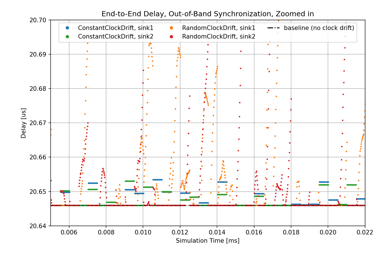
In the case of the constant clock drift, the drift rate difference is compensated perfectly at the first synchronization event, thus the line sections are completely horizontal. However, we specified a random error for the time difference synchronization, thus the values change at every synchronization event, every 0.5ms.
In the case of the random clock drift, the drift rate is compensated with no error at every synchronization event, but the drift rate of the clocks keeps changing randomly even between synchronization events. This results in fluctuating delay.
Let’s see the case where a random clock drift rate oscillator is used with gPTP:
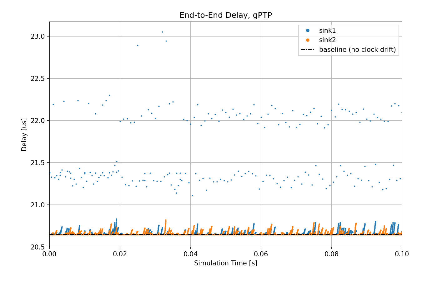
The delay distribution is similar to the out-of-band synchronization case, but
there are outliers. gPTP needs to send packets over the network for time
synchronization, as opposed to using an out-of-band mechanism. These gPTP
messages can sometimes cause delays for packets from source1, causing them
to wait in the queue.
Note
The outliers can be eliminated by giving gPTP packets priority over the source application packets. Ideally, they can have allocated time in the gate schedule as well.
The following chart displays out-of-band synchronization and gPTP, so they can be compared:
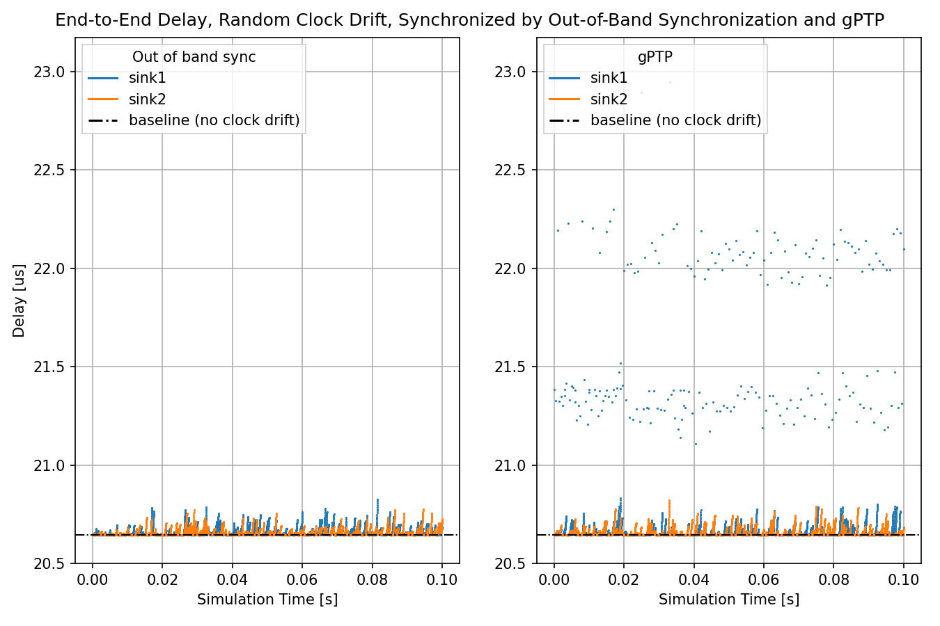
In all these cases, the applications send packets in sync with the opening of
the gates in the queue in switch1. In the no clock drift case, the delay
depends only on the bit rate and packet length. In the case of
OutOfBandSynchronization and GptpSynchronization, the clocks drift but
the drift is periodically eliminated by synchronization, so the delay remains
bounded.
Let’s see what happens to delay when there is no synchronization:
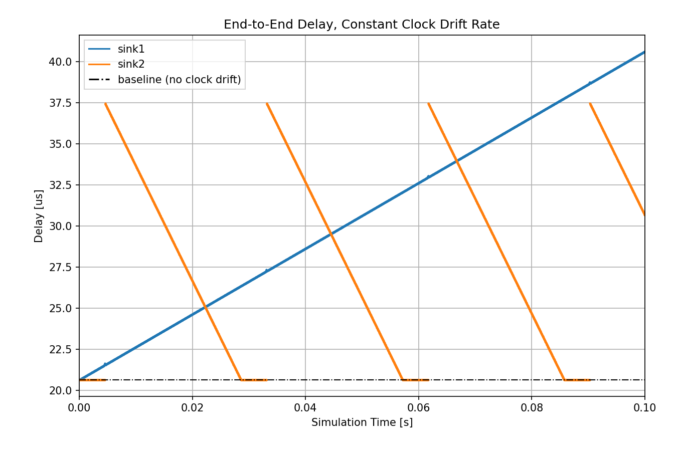
The delay keeps changing substantially compared to the other cases.
What’s the reason behind these graphs? When there is no clock drift (or it is
eliminated by synchronization), the end-to-end delay is bounded because the
packets are generated in the sources in sync with the opening of the
corresponding gates in switch1 (the send windows). In the constant clock
drift case, the delay’s characteristics depend on the magnitude and direction of
the drift between the clocks.
It might be helpful to think of the constant drift rate as time dilation. In
ideal conditions (no clock drift or eliminated clock drift), the clocks in all
three modules keep the same time, so there is no time dilation. The packets in
both sources are generated in sync with the send windows (when the corresponding
gate is open), and they are forwarded immediately by switch1. In the
constant clock drift case, from the point of view of switch1, the clock of
source1 is slower than its own, and the clock of source2 is faster.
Thus, the packet stream from source1 is sparser than in the ideal case, and
the packet stream from source2 is denser, due to time dilation.
If the packet stream is sparser (orange graph), there are on average fewer
packets to send than the number of send windows in a given amount of time, so
packets don’t accumulate in the queue. However, due to the drifting clocks, the
packet generation and the send windows are not in sync anymore but keep
shifting. Sometimes a packet arrives at the queue in switch1 when the
corresponding gate is closed, so it has to wait for the next opening. This next
opening happens earlier and earlier for subsequent packets (due to the relative
direction of the drift in the two clocks), so packets wait less and less in the
queue, hence the decreasing part of the curve. Then the curve becomes
horizontal, meaning that the packets arrive when the gate is open and they can
be sent immediately. After some time, the gate opening shifts again compared to
the packet generation, so the packets arrive just after the gate is closed, and
they have to wait for a full cycle in the queue before being sent.
If the packet stream is denser (blue graph), there are more packets to send on average than the number of send windows in a given amount of time, so packets eventually accumulate in the queue. This causes the delay to keep increasing indefinitely.
Note
The packets are not forwarded by
switch1if the transmission wouldn’t finish before the gate closes (a packet takes 6.4us to transmit, the gate is open for 10us).The length of the horizontal part of the orange graph is equal to how much the two clocks drift during the time of
txWindow - txDuration. In the case of the orange graph, it is(10us - 6.4us) / 700ppm ~= 5ms
Thus, if constant clock drift is not eliminated, the network can no longer guarantee any bounded delay for the packets. The constant clock drift has a predictable repeated pattern but still has a significant effect on delay.
Let’s examine the random clock drift case:
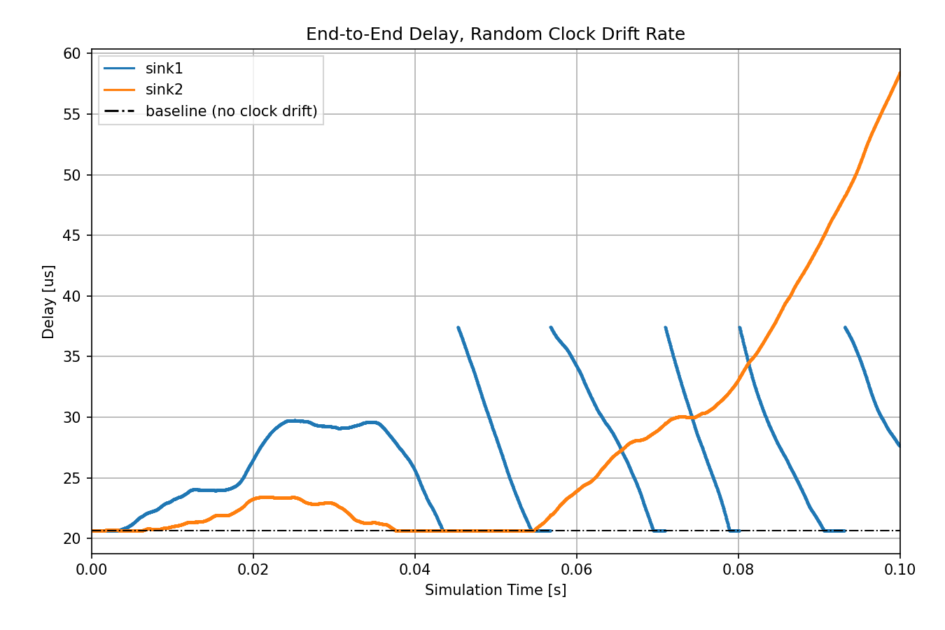
Unpredictable random clock drift might have an even larger impact on delay.
The following chart compares the constant and random clock drift rate cases:
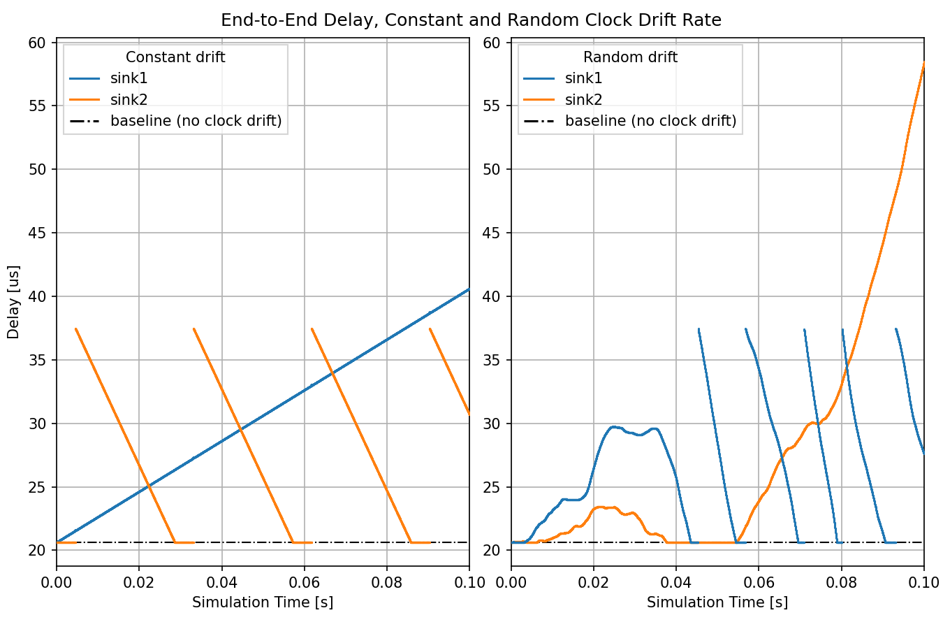
The clocks in the similar plots (e.g., constant drift/sink1 and random drift/sink2) drift in the same direction.
Sources: omnetpp.ini, ClockDriftShowcase.ned
Try It Yourself
If you already have INET and OMNeT++ installed, start the IDE by typing
omnetpp, import the INET project into the IDE, then navigate to the
inet/showcases/tsn/timesynchronization/clockdrift folder in the Project Explorer. There, you can view
and edit the showcase files, run simulations, and analyze results.
Otherwise, there is an easy way to install INET and OMNeT++ using opp_env, and run the simulation interactively.
Ensure that opp_env is installed on your system, then execute:
$ opp_env run inet-4.6 --init -w inet-workspace --install --build-modes=release --chdir \
   -c 'cd inet-4.6.*/showcases/tsn/timesynchronization/clockdrift && inet'
This command creates an inet-workspace directory, installs the appropriate
versions of INET and OMNeT++ within it, and launches the inet command in the
showcase directory for interactive simulation.
Alternatively, for a more hands-on experience, you can first set up the workspace and then open an interactive shell:
$ opp_env install --init -w inet-workspace --build-modes=release inet-4.6
$ cd inet-workspace
$ opp_env shell
Inside the shell, start the IDE by typing omnetpp, import the INET project,
then start exploring.
Discussion
Use this page in the GitHub issue tracker for commenting on this showcase.