Using Traffic Shapers Independently
Goals
Within the INET framework, scheduling and traffic shaping modules can operate independently from a network node. Leveraging these modules in this manner offers the advantage of easily constructing and verifying intricate scheduling and traffic shaping behaviors that may be challenging to replicate within a comprehensive network setup.
In this showcase, we demonstrate the creation of a fully operational Asynchronous Traffic Shaper (ATS) by directly interconnecting its individual components. Next, we construct a straightforward queuing network by linking the ATS to traffic sources and traffic sinks. The key highlight is the observation of traffic shaping within the network, achieved by plotting the generated traffic both before and after the shaping process.
4.6Asynchronous Traffic Shaping in INET
The Asynchronous Traffic Shaper, as defined in the IEEE 802.1Qcr standard, effectively smooths traffic flow by capping the data rate to a nominal value while permitting certain bursts. In INET, this mechanism is realized through four essential modules:
EligibilityTimeMeter: Calculates the transmission eligibility time, determining when a packet becomes eligible for transmission.
EligibilityTimeFilter: Filters out expired packets, those that would wait excessively before becoming eligible for transmission.
EligibilityTimeQueue: Stores packets in order of their transmission eligibility time.
EligibilityTimeGate: Opens at the transmission eligibility time for the next packet.
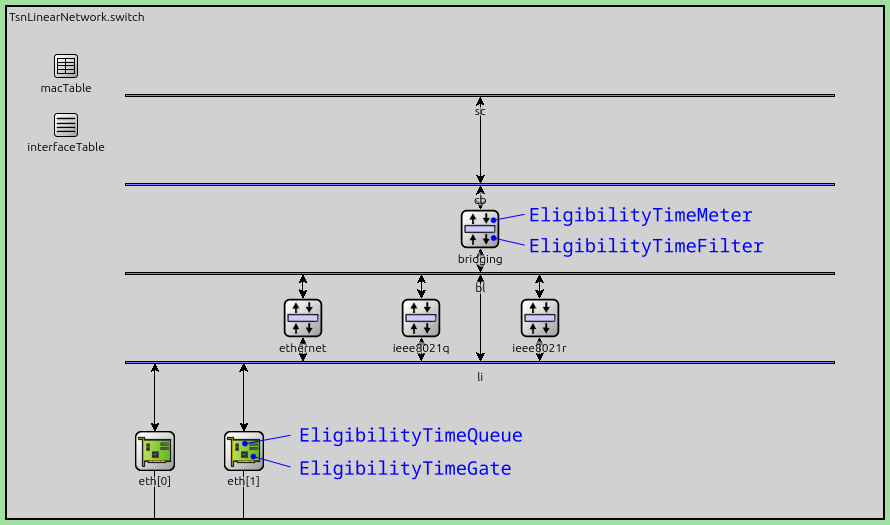
In a complete network setup, these modules are typically distributed across various components of a network node, such as an Ethernet switch. Specifically, the meter and filter modules are positioned within the ingress filter of the bridging layer, while the queue and gate modules reside in the network interfaces. Refer to the annotated image of a TsnSwitch below for a visual representation of their locations:
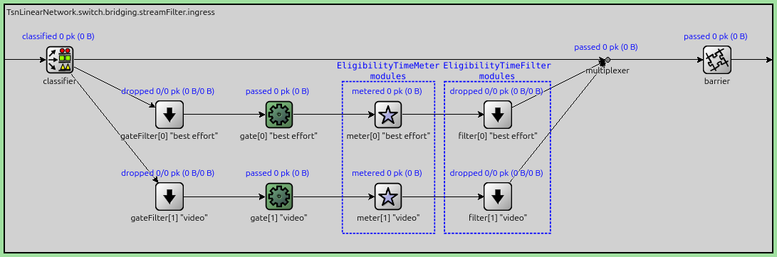
The next image displays an internal view of the ingress filter module in the bridging layer of the switch, with the EligibilityTimeQueue and the EligibilityTimeFilter modules highlighted:
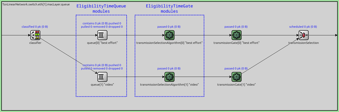
The following image displays an internal view of the queue module in the Ethernet interface’s MAC layer, with the EligibilityTimeQueue and EligibilityTimeGate modules highlighted:
Note
For more comprehensive information on ATS in a complete network and additional details about ATS configuration, please refer to the Asynchronous Traffic Shaping showcase.
The Model
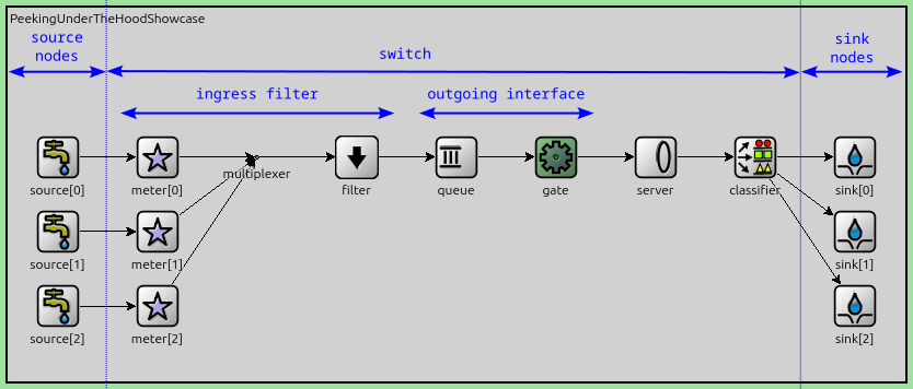
In the next sections, we present a simulation model, which demonstrates how ATS components can be used outside INET network nodes. The network is depicted in the following image:
The queuing network includes three independent packet sources, each linked to an EligibilityTimeMeter, ensuring individual data rate metering for each packet stream. These meters are then connected to a single EligibilityTimeFilter module that drops expired packets.
Subsequently, the filter is linked to an EligibilityTimeQueue, effectively organizing packets based on their transmission eligibility time. From there, the queue is connected to an EligibilityTimeGate, which opens to allow packets through in accordance with their transmission eligibility time.
Finally, the gate connects to a server responsible for periodically pulling packets from the queue while the gate is open. The server then sends these packets to one of the packet sinks via a classifier, which separates the three streams.
Note
Although there is only one filter, queue, and gate module, the three packet streams are still individually shaped. This is made possible because the transmission eligibility time is calculated per-stream by the three meters.
Traffic
The packet sources generate traffic with different sinusoidal production rates:
*.numSources = 3
*.source[*].packetLength = 1000B
*.source[0].productionInterval = replaceUnit(sin(dropUnit(simTime() * 2)) + 5, "ms") / 10
*.source[1].productionInterval = replaceUnit(sin(dropUnit(simTime() * 3)) + 5, "ms") / 10
*.source[2].productionInterval = replaceUnit(sin(dropUnit(simTime() * 1)) + sin(dropUnit(simTime() * 8)) + 5, "ms") / 10
Traffic Shaping
To configure the traffic shaping, we specify the committed information rate and burst size parameters in the meter modules. Additionally, we set a maximum residence time in the meter, which enables the filter to discard packets that would otherwise wait excessively in the queue before becoming eligible for transmission.
The active server module pulls packets from the traffic shaper when the gate allows it. We set a constant processing time for each packet in the server, so the server tries to pull packets every 0.1ms:
*.meter[*].committedInformationRate = 16Mbps
*.meter[*].committedBurstSize = 10kB
*.meter[*].maxResidenceTime = 10ms

*.server.processingTime = 0.1ms
Classifying
To measure and plot the post-shaping data rates of the individual streams,
we need to separate them.
To that end, we set up the classifier to
make traffic flow from each source to its sink counterpart (i.e. source[0] ->
sink[0] and so on). The classifier is a ContentBasedClassifier.
It classifies packets by name, which contains the name of the source
module:
To measure and plot the post-shaping data rates of individual
streams, we require their separation. For this purpose, we configure the
classifier to route traffic from each source to its corresponding sink (e.g.,
source[0] -> sink[0], source[1] -> sink[1], and so on). Utilizing the
ContentBasedClassifier, we classify packets based on their names, which include
the source module’s name:
*.classifier.packetFilters = ["source[0]*", "source[1]*", "source[2]*"]
Note
In a complete network setup, managing streams involves several features, such as stream identification, encoding, and decoding. Typically, packets would be assigned to specific streams using VLAN IDs or PCP (Priority Code Point) numbers.
Results
Let’s examine the data rate of the corresponding source-sink pairs. We’ll observe the traffic from the sources and compare it to the traffic arriving at the sinks after the shaping process:
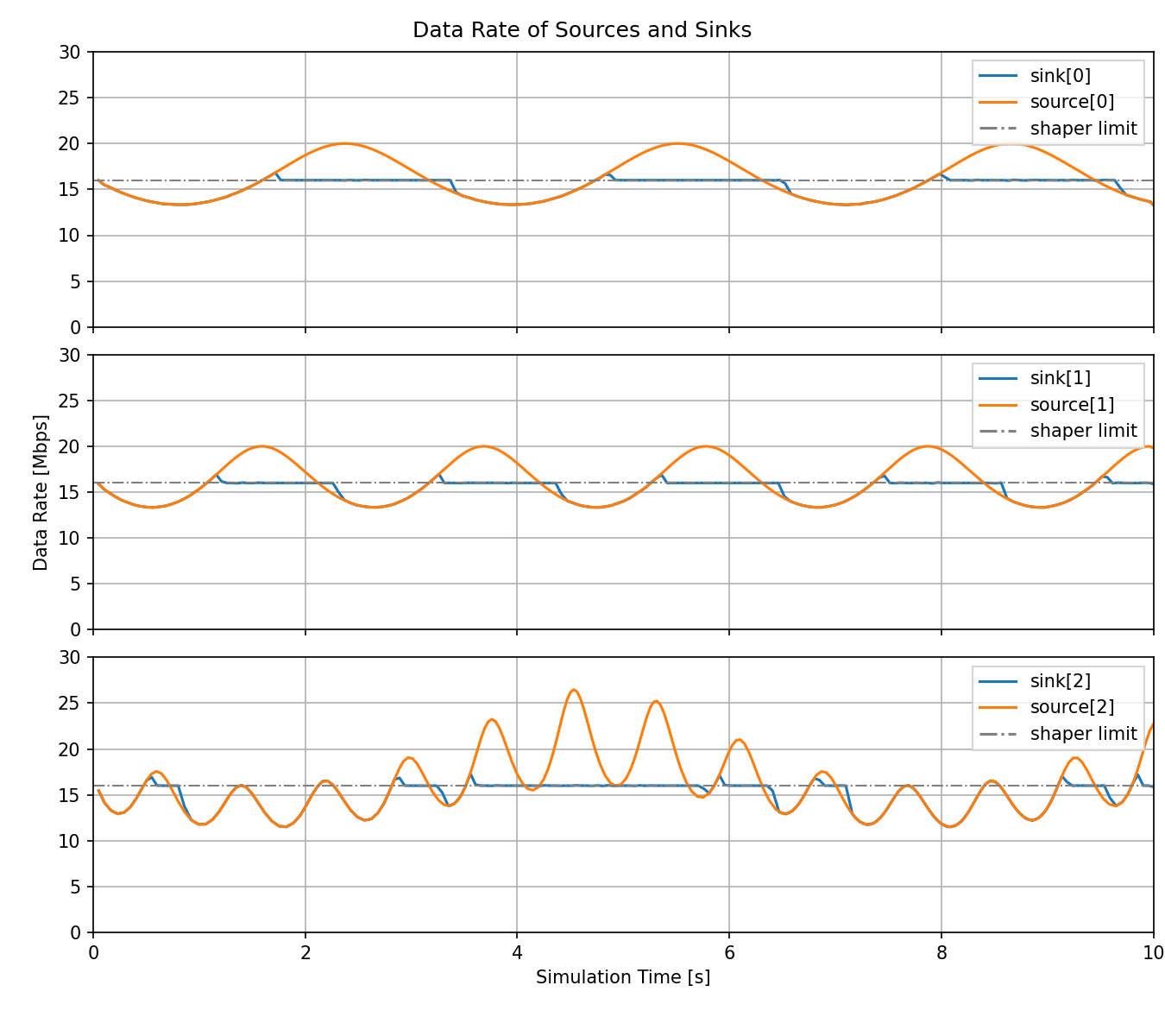
The data rate of the sinusoidal source traffic occasionally exceeds the 16Mbps per-stream shaper limit. However, the shaper does allow a brief burst before limiting the traffic to the configured limit.
Next, we’ll examine the relationship between traffic before and after shaping, as well as the packet drop rate. Due to having only one filter, we are limited to presenting the sum of dropped packets for all streams. Consequently, we will display the same data as on the earlier plots but consolidate all streams onto a single chart. Additionally, we will include the packet drop rate of the filter module to provide a comprehensive overview of the shaping process.
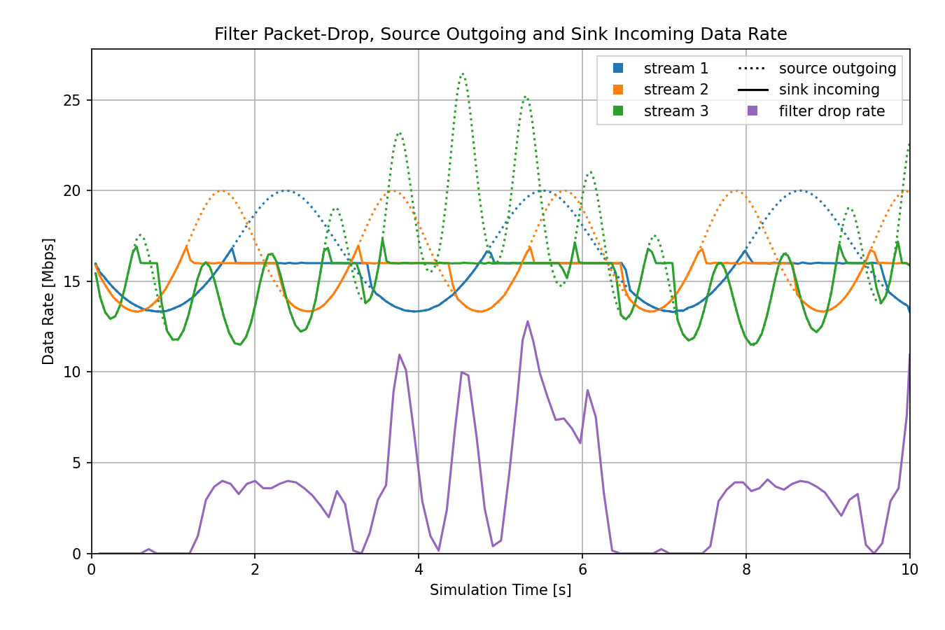
Despite the presence of a single combined shaper in the network (comprising one filter, queue, and gate), each stream is individually limited to 16Mbps due to separate metering. Notably, we can observe a higher packet drop rate when the source traffic exceeds the per-stream shaper limit.
Note that as traffic increases above the shaper limit, first some packets are stored in the queue to be sent later. If the traffic stays above the shaper limit, some packets would have to wait in the queue for longer than the max residence time, so the filter drops these excess packets. The drop rate roughly follows the incoming traffic rate.
The next chart shows how the queueing time changes:
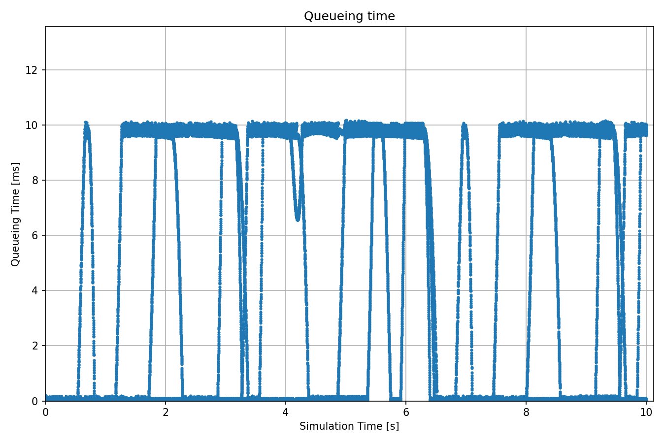
The maximum of the queueing time is 10ms, which is due to the max residence time set in the filter. Packets that would wait longer in the queue are dropped by the filter before getting there.
Note
The chart above might give the appearance of three data series plotted with the same color. This is because the streams are metered separately, but the filter doesn’t distinguish them.
The next chart shows the queue length:
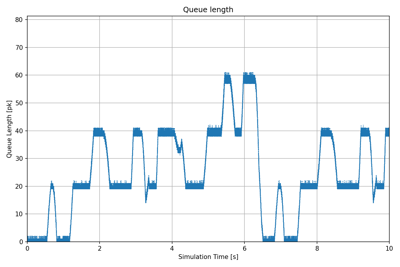
The maximum number of packets that can accumulate in the queue from each stream is 20, calculated as follows: max residence time / average production interval = 10ms / 0.5ms = 20. Since the traffic pattern is different for the three streams, the 20 packets/stream limit is reached at different times for each of them. We can observe on the chart as the queue becomes saturated for each stream individually. The maximum of the queue length is 60, when all streams reach their maximum packet count in the queue.
Sources: omnetpp.ini, PeekingUnderTheHoodShowcase.ned
Try It Yourself
If you already have INET and OMNeT++ installed, start the IDE by typing
omnetpp, import the INET project into the IDE, then navigate to the
inet/showcases/tsn/trafficshaping/underthehood folder in the Project Explorer. There, you can view
and edit the showcase files, run simulations, and analyze results.
Otherwise, there is an easy way to install INET and OMNeT++ using opp_env, and run the simulation interactively.
Ensure that opp_env is installed on your system, then execute:
$ opp_env run inet-4.6 --init -w inet-workspace --install --build-modes=release --chdir \
   -c 'cd inet-4.6.*/showcases/tsn/trafficshaping/underthehood && inet'
This command creates an inet-workspace directory, installs the appropriate
versions of INET and OMNeT++ within it, and launches the inet command in the
showcase directory for interactive simulation.
Alternatively, for a more hands-on experience, you can first set up the workspace and then open an interactive shell:
$ opp_env install --init -w inet-workspace --build-modes=release inet-4.6
$ cd inet-workspace
$ opp_env shell
Inside the shell, start the IDE by typing omnetpp, import the INET project,
then start exploring.
Discussion
Use this page in the GitHub issue tracker for commenting on this showcase.