Power Consumption
Goals
Power consumption is a critical aspect of the design and operation of wireless networks, particularly in mobile and energy-constrained systems. In this showcase, we demonstrate how to model the energy consumption, energy storage, and energy generation of mobile nodes in an ad-hoc wireless network. Through an example simulation, we will examine the impact of wireless communication on the power consumption of the mobile nodes, with the main focus being on the energy consumed by the radio. The modeled devices also have energy storage units (batteries) and energy generation units (modeling solar cells) built into them.
4.6The model
The network
The network consists of a configurable number of stationary wireless nodes of the type AdhocHost. The hosts are placed on the scene randomly at the start of the simulation. The radios are configured so that hosts can reach each other in one hop, so no routing is needed. We’ll use the ping application in each host to generate network traffic. During the simulation, radios will draw power from the nodes’ energy storage units, while power generators will charge them. After the simulation has finished, we will analyze the recorded energy storage statistics.
The simulations will be run using 20 hosts. Here is what the network will look like when the simulation is run:

Configuration and behavior
All hosts are configured to ping host[0] every second. host[0]
doesn’t send ping requests, just replies to the requests that it
receives. To reduce the probability of collisions, the ping
application’s start time is chosen randomly for each host as a value
between 0 and 1 seconds. Since ping requests have a short duration and
hosts transmit infrequently, it is assumed that the probability of
collisions will be very low.
Energy Storage, Generation, and Management
Hosts are configured to contain a SimpleEpEnergyStorage module.
SimpleEpEnergyStorage keeps a record of stored energy in Joules, and
power input/output in Watts. The letters Ep stand for energy and
power, denoting how the module represents energy storage and power
input/output. There are other energy storage models in INET that,
similarly to real batteries, use charge and current (denoted by Cc),
such as SimpleCcBattery. SimpleEpEnergyStorage models energy
storage by integrating the difference between absorbed and provided power
over time. It does not simulate other effects of real batteries, such as
temperature dependency and hysteresis. It is used in this model because
the emphasis is on the energy that transmissions use, not how the
batteries store the energy. Each host is configured to have a nominal
energy storage capacity of 0.05 Joules. The charge they contain at the
beginning of the simulation is randomly selected between zero and the
nominal capacity for each host.
Each host contains an AlternatingEpEnergyGenerator module. This module
alternates between generation (active) and sleep states. It starts in
the generation state, and while there, it generates the power that is
specified in its powerGeneration parameter (now set to 4mW). In the
sleep state, it generates no power. It stays in each mode for the
durations specified in the generationInterval and sleepInterval
parameters. These are set to a random value with a mean of 25s for each
host.
Energy storage and generator modules are controlled by energy management
modules. In this showcase, hosts are configured to contain a
SimpleEpEnergyManagement module. We configure energy management
modules to shut down hosts when their energy levels reach 10% of the
nominal capacity (0.005 Joules) and restart them when their energy
storage charges to half of their nominal energy capacity, i.e. 0.025
Joules. These settings can be specified in the energy management
module’s nodeShutdownCapacity and nodeStartCapacity parameters.
Radio modes and states
In the Ieee80211Radio model used in this simulation (and in other radio models), there are different modes in which radios operate, such as off, sleep, receiver, and transmitter. The mode is set by the model and does not depend on external effects. In addition to mode, radios have states, which depend on what they are doing in the given mode – i.e. listening, receiving a transmission, or transmitting. The state depends on external factors, such as if there are transmissions going on in the medium.
Energy consumption of radios
Radios in the simulation are configured to contain a StateBasedEpEnergyConsumer module. In this model, energy consumption is based on power consumption values for various radio modes and states, and the time the radio spends in these states. For example, radios consume a small amount of power when they are idle in receive mode, i.e. when they are listening for transmissions. They consume more power when they are receiving a transmission, and even more when they are transmitting.
Energy storage visualization
The energy storage capacity of nodes can be visualized by the EnergyStorageVisualizer module, which displays a battery icon next to the nodes, indicating their charge levels. This visualizer is included in the network as part of the IntegratedCanvasVisualizer module.
Results
The following video has been captured from the simulation. The gauges next to each host indicate energy levels, and a red “x” on a host’s icon means that the host is down. Note how energy levels change while the simulation is running.
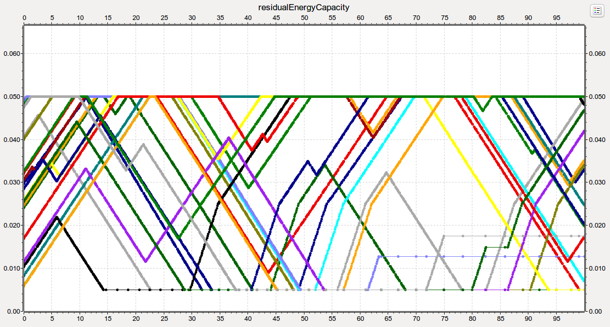
The following plot shows the energy storage levels of all the hosts
through the course of the simulation, recorded as the
residualEnergyCapacity statistic. We can see that each host starts
from a given charge level, and their energy levels constantly decrease
from there. It eventually reaches the shutdown capacity, and when that
happens, the host shuts down. Then it starts to charge, and when the
charge level reaches the 0.025J threshold, the host turns back on.
The generator generates more power than hosts consume when they are idle, but not when they are receiving or transmitting. This difference appears on the graph as increasing curves when the generator is charging, with tiny zigzags associated with receptions and transmissions. When hosts get fully charged, they maintain the maximum charge level while the generator is charging.
The plot below shows the energy storage level (red curve) and the energy
generator output (blue curve) of host[12]. The intervals when the
generator is charging the energy storage can be discerned on the energy
storage graph as increasing slopes. When the host is transmitting and
the generator is charging, the energy levels don’t increase as fast. The
generator generates 4mW of power, and radios consume 2mW when they are
idle in receiver mode. Radios are in the idle state most of the time, thus
their power consumption is roughly 2mW. When the host is up and being
charged, the net charge is 2mW (4mW provided by the generator and 2mW
consumed by the radio). When the host is down and being charged, the net
charge is 4mW. The latter corresponds to the most steeply increasing
curve sections. When the host is up but not charging, the consumption is
2mW, and the curve is decreasing.
The tiny zigzags in the graph when the host is up are because of the increased power consumption associated with transmitting (it requires 100mW of power). In the intervals when the host is down, the curve is smooth (there are still some drawing artifacts due to multiple line segments, but that can be ignored).

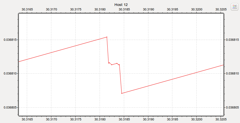
The following plot shows how the energy level of host[12] changes
during a transmission while charging.
host[0] is different from the other hosts in that it doesn’t send
ping requests, it “only” sends replies to the pings sent by the other
hosts. (Hosts send one ping request every second.) Note that although
host[0] transmits around 20 times more than the other hosts, its
energy consumption is similar to the other hosts’ (host[0] is the
blue curve). This is so because is its energy consumption is still
dominated by reception: the host spends most of its time listening, and
only a fraction of time transmitting.

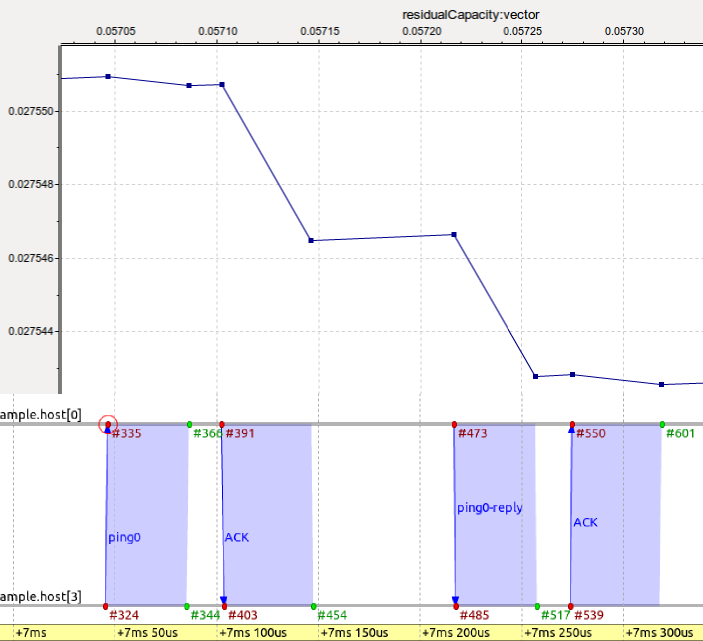
The following plot shows a ping request-ping reply exchange (with the
associated ACKs) between hosts 0 and 3 on the sequence chart and the
corresponding changes in energy levels of host[0]. Note that
host[0] consumes less energy receiving than transmitting. In the
intervals between the transmissions, the curve is increasing because
the generator is charging host[0]. This image shows that hosts
indeed consume more power when transmitting than the generator
generates. However, transmissions are very short and very rare, so one
needs to zoom in on the graph to see this effect.
Sources: omnetpp.ini, PowerConsumptionShowcase.ned
Try It Yourself
If you already have INET and OMNeT++ installed, start the IDE by typing
omnetpp, import the INET project into the IDE, then navigate to the
inet/showcases/wireless/power folder in the Project Explorer. There, you can view
and edit the showcase files, run simulations, and analyze results.
Otherwise, there is an easy way to install INET and OMNeT++ using opp_env, and run the simulation interactively.
Ensure that opp_env is installed on your system, then execute:
$ opp_env run inet-4.6 --init -w inet-workspace --install --build-modes=release --chdir \
   -c 'cd inet-4.6.*/showcases/wireless/power && inet'
This command creates an inet-workspace directory, installs the appropriate
versions of INET and OMNeT++ within it, and launches the inet command in the
showcase directory for interactive simulation.
Alternatively, for a more hands-on experience, you can first set up the workspace and then open an interactive shell:
$ opp_env install --init -w inet-workspace --build-modes=release inet-4.6
$ cd inet-workspace
$ opp_env shell
Inside the shell, start the IDE by typing omnetpp, import the INET project,
then start exploring.
Discussion
Use this page in the GitHub issue tracker for commenting on this showcase.