Modeling Directional Antennas
Goals
Modeling directional antennas refers to the use of antenna models in simulations to represent the directional characteristics of real-world antennas. Directional antennas are designed to transmit and receive signals in a specific direction, rather than uniformly in all directions. This can be useful in a variety of wireless scenarios where the directionality of the antenna is important, such as in long-range communication.
INET contains various models of directional antennas, which can be used to simulate different types of antenna patterns. In this showcase, we will highlight the antenna models that are available in INET and provide an example simulation that demonstrates the directionality of five different antenna models. Four of these models represent well-known antenna patterns, while the fifth model is a universal antenna that can be used to model any rotationally symmetrical antenna pattern. By the end of this showcase, you will understand the different antenna models available in INET and how they can be used to simulate the directionality of antennas.
4.6Concepts
In INET, radio modules contain transmitter, receiver, and antenna submodules. The success of receiving a wireless transmission depends on the strength of the signal present at the receiver, among other things, such as interference from other signals. Both the transmitter and the receiver submodules use the antenna submodule of the radio when sending and receiving transmissions.
The antenna module affects transmission and reception in multiple ways:
The relative position of the transmitting and receiving antennas is used when calculating reception signal strength (e.g. attenuation due to distance).
Antenna gain is applied to the signal power at transmission and reception. The applied gain depends on each antenna module’s directional characteristics, and the relative position and the orientation of the two antennas. The gain can increase or decrease the received signal power.
By default, the antenna uses the containing network node’s mobility submodule to describe its position and orientation, i.e. it has the same position and orientation as the network node. However, antenna modules have optional mobility submodules of their own.
All antenna modules have 3D directional characteristics.
INET contains the following antenna module types:
Isotropic:
IsotropicAntenna: hypothetical antenna that radiates with the same intensity in all directions
ConstantGainAntenna: the same as IsotropicAntenna, but has a constant gain parameter (for testing purposes)
Omnidirectional:
DipoleAntenna: models a dipole antenna
Directional:
ParabolicAntenna: models a parabolic antenna’s main radiation lobe, ignoring sidelobes
CosineAntenna: models directional antenna characteristics with a cosine pattern
Other:
AxiallySymmetricAntenna: can model arbitrary antennas with axially symmetric radiation patterns
InterpolatingAntenna: can model antennas with arbitrary radiation patterns, using interpolation
The default antenna module in all radios is IsotropicAntenna.
Visualizing Antenna Directionality
The RadioVisualizer module can visualize antenna directional characteristics, using its antenna lobe visualization feature. For example, the radiation patterns of an isotropic and a directional antenna look like the following:
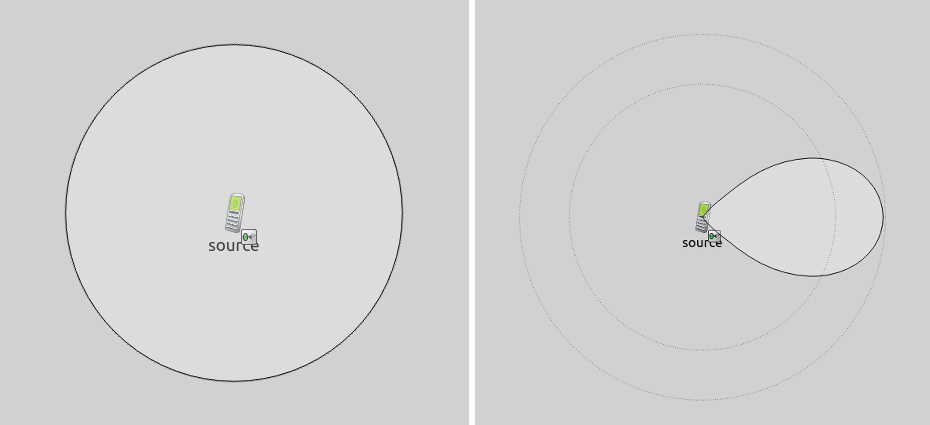
The visualized lobes indicate the antenna gain. At any given direction, the distance between the node and the boundary of the lobe shape is a (linear or logarithmic, the default being the latter) function of the gain in that direction. Details of the mapping can be tuned with the visualizer’s parameters. Dashed circles indicate the 0 dB gain and the maximum gain on the radiation pattern figure.
The visualization is actually a cross-section of the 3D radiation pattern. By default, the cross-section plane is perpendicular to the current viewing angle (however, one can specify other planes in the antenna’s local coordinate system).
For the description of all parameters of the visualizer, check the NED documentation of RadioVisualizerBase.
The Model and Results
The showcase contains five example simulations, which demonstrate the
directional characteristics of five antenna models. The simulation uses
the DirectionalAntennasShowcase network:
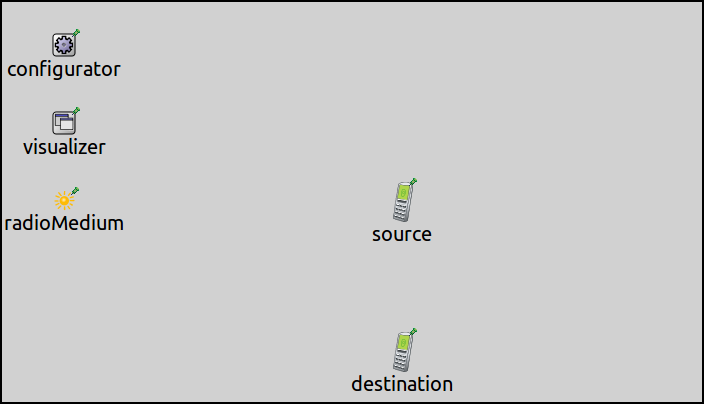
The network contains two AdhocHost s, named source and
destination. There is also an Ipv4NetworkConfigurator, an
IntegratedCanvasVisualizer, and an Ieee80211RadioMedium module.
The source host is positioned in the center of the playground. The
destination host is configured to circle the source host, while the
source host pings the destination every 0.5 seconds. We’ll use the ping
transmissions to probe the directional characteristics of source’s
antenna, by recording the power of the received signal in
destination. The destination host will do one full circle around the
source. The distance of the two hosts will be constant to get meaningful
data about the antenna characteristics. We’ll run the simulation with
five antenna types in source: IsotropicAntenna,
ParabolicAntenna, DipoleAntenna, CosineAntenna, and
AxiallySymmetricAntenna. The destination has the default
IsotropicAntenna in all simulations.
The configurations for the five simulations differ in the antenna
settings only; all other settings are in the General configuration
section:
[General]
network = DirectionalAntennasShowcase
sim-time-limit = 360s
abstract = true

# don't send arp messages
*.*.ipv4.arp.typename = "GlobalArp"

# ping app settings
*.source.numApps = 1
*.source.app[0].typename = "PingApp"
*.source.app[0].destAddr = "destination"
*.source.app[0].sendInterval = 0.5s

# mobility settings
*.destination.mobility.typename = "CircleMobility"
*.destination.mobility.cx = 400m
*.destination.mobility.cy = 200m
*.destination.mobility.r = 150m
*.destination.mobility.startAngle = 90deg
*.destination.mobility.speed = -2.61799387799mps

# visualizer settings
*.visualizer.radioVisualizer.displayRadios = true
*.visualizer.radioVisualizer.displayAntennaLobes = true
*.visualizer.radioVisualizer.radioFilter = "*.source**"
*.visualizer.dataLinkVisualizer.displayLinks = true
The source host is configured to send ping requests every 0.5s. This is
effectively the probe interval; the antenna characteristics data can be
made more fine-grained by setting a more frequent ping rate. The
destination is configured to circle the source with a radius of 150m.
The simulation runs for 360s, and the speed of destination is set so
it does one full circle. This way, when plotting the reception power,
the time can be directly mapped to the angle.
The visualizer is set to display antenna lobes in source (the
displayRadios is the master switch in RadioVisualizer, so it
needs to be set to true), and active data links (indicating successfully received
transmissions).
The antenna specific settings are defined in distinct configurations,
named according to the antenna type used (IsotropicAntenna,
ParabolicAntenna, DipoleAntenna, CosineAntenna, and
AxiallySymmetricAntenna).
Isotropic Antenna
The IsotropicAntenna is the default in all radio modules. This
module models a hypothetical antenna which radiates with the same power
in all directions. The module has no parameters. The
simulation configuration which demonstrates this antenna is IsotropicAntenna in omnetpp.ini.
The configuration just sets the antenna type in source:
[Config IsotropicAntenna]

*.source.wlan[*].radio.antenna.typename = "IsotropicAntenna"
When the simulation is run, it looks like the following:
The radiation pattern is shown as a circle, as expected (the isotropic antenna’s radiation pattern is a sphere).
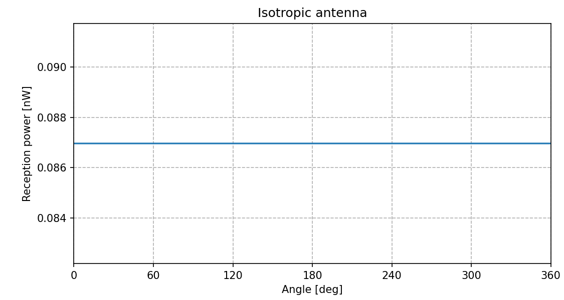
As the destination node circles the source node, we record the reception power of the frames. Here is the reception power vs. direction plot:
Parabolic Antenna
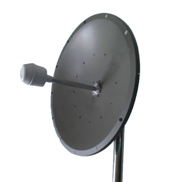
The ParabolicAntenna module simulates the radiation pattern of the main lobe of a parabolic antenna, such as this one:
The antenna module has the following parameters:
maxGain: the maximum gain of the antenna in dBminGain: the minimum gain of the antenna in dBbeamWidth: width of the 3 dB beam in degrees
The configuration for this antenna is ParabolicAntenna in
omnetpp.ini:
[Config ParabolicAntenna]

*.source.wlan[*].radio.antenna.typename = "ParabolicAntenna"
*.source.wlan[*].radio.antenna.beamWidth = 30deg
*.source.wlan[*].radio.antenna.maxGain = 10dB
*.source.wlan[*].radio.antenna.minGain = -50dB
When the simulation is run, it looks like the following:
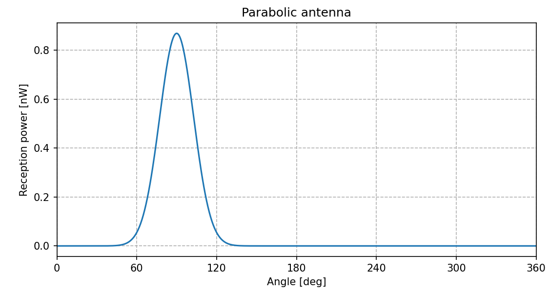
The radiation pattern is a narrow lobe. Note that in directions away from the main direction, the radiation pattern might appear to be zero, but actually, it is just very small. Note the small protrusion to the left on the following, zoomed-in image:

The ping probe messages are successfully received when the destination
node is near the main lobe of source’s antenna.
Here is the reception power vs. direction plot (note that the destination host
starts at 90 degrees away from the main lobe axis, so that the main lobe is
more apparent on the reception power plot):
Dipole Antenna
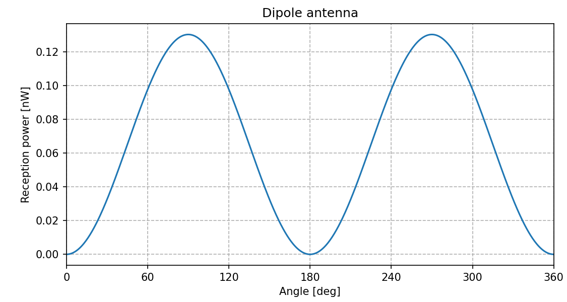
The DipoleAntenna module models a dipole antenna. Antenna length can be specified with
a parameter. By default, the antenna is vertical. When viewed from above, its radiation pattern
is a circle, which would not be very interesting for demonstration. To make the simulation
more interesting, we set the antenna to point in the direction of the y axis.
The configuration in omnetpp.ini is the
following:
[Config DipoleAntenna]

*.source.wlan[*].radio.antenna.typename = "DipoleAntenna"
*.source.wlan[*].radio.antenna.length = 0.1m
*.source.wlan[*].radio.antenna.wireAxis = "y"
It looks like this when the simulation is run:
The visualization shows the cross-section of the donut shape of the dipole antenna’s radiation pattern. As can be seen from the animation, there is no successful communication when the destination node is near the antenna’s axis due to low antenna gain in that direction. Here is the reception power vs. direction plot:
Cosine Antenna
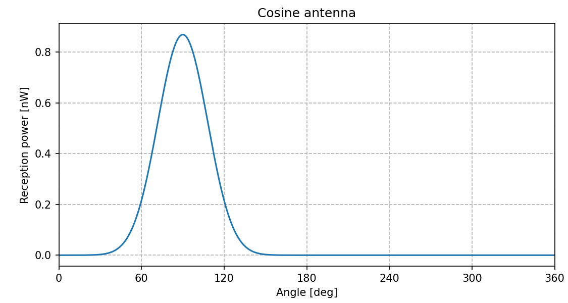
The CosineAntenna module models a hypothetical antenna with a cosine-based
radiation pattern. This antenna model is commonly used in the real world to approximate
various directional antennas. The module has two parameters, maxGain
and beamWidth. The configuration in omnetpp.ini is the
following:
[Config CosineAntenna]

*.source.wlan[*].radio.antenna.typename = "CosineAntenna"
*.source.wlan[*].radio.antenna.beamWidth = 30deg
*.source.wlan[*].radio.antenna.maxGain = 10dB
It looks like the following:
As can be seen on the video, the radiation pattern is similar to that of the parabolic antenna. Here is the reception power vs. direction plot:
Axially Symmetric Antenna
The AxiallySymmetricAntenna is a universal antenna model which can describe any axially symmetrical radiation pattern. It can model an isotropic antenna, a parabolic antenna, dipole antenna, and many other antenna types.
The radiation pattern is described by specifying the gain at various angles on a half-plane attached to the axis of symmetry. The gain is then interpolated at the intermittent angles, and the pattern is rotated around the axis to get the radiation pattern in 3D.
The antenna module has three parameters:
the gains parameter takes a sequence of gain and angle pairs
(given in decibels and degrees), the first pair must be 0 0.
The angle is in the range of (0,180).
The axis of symmetry is given by the axisOfSymmetry parameter, x by default.
There is also a baseGain parameter (0 dB by default). The default for the gains
parameters is "0 0", defaulting to an isotropic antenna.
We demonstrate AxiallySymmetricAntenna by modeling a real-world 16-element Yagi antenna, such as this one:

The antenna type in source’s radio is set to
AxiallySymmetricAntenna. We entered the characteristics data for the antenna
in the gains parameter with 1 degree resolution.
We also set a baseGain of 10 dB, because the gain data is given as relative
(i.e. the maximum gain is at 0 dB).
The simulation configuration is AxiallySymmetricAntenna in
omnetpp.ini:
[Config AxiallySymmetricAntenna]

*.source.wlan[*].radio.antenna.typename = "AxiallySymmetricAntenna"
*.source.wlan[*].radio.antenna.baseGain = 10dB
*.source.wlan[*].radio.antenna.gains = "0 0.000 1 -0.010 2 -0.039 3 -0.088 4 -0.156 5 -0.245 6 -0.354 7 -0.484 8 -0.635 9 -0.807 10 -1.002 11 -1.220 12 -1.461 13 -1.727 14 -2.019 15 -2.336 16 -2.680 17 -3.051 18 -3.451 19 -3.880 20 -4.338 21 -4.826 22 -5.344 23 -5.890 24 -6.464 25 -7.064 26 -7.687 27 -8.328 28 -8.982 29 -9.641 30 -10.299 31 -10.945 32 -11.572 33 -12.172 34 -12.740 35 -13.276 36 -13.786 37 -14.277 38 -14.766 39 -15.267 40 -15.801 41 -16.389 42 -17.053 43 -17.816 44 -18.707 45 -19.757 46 -21.009 47 -22.517 48 -24.356 49 -26.624 50 -29.385 51 -32.255 52 -33.256 53 -31.393 54 -28.954 55 -26.957 56 -25.451 57 -24.345 58 -23.561 59 -23.044 60 -22.758 61 -22.678 62 -22.789 63 -23.081 64 -23.548 65 -24.188 66 -24.994 67 -25.956 68 -27.048 69 -28.212 70 -29.338 71 -30.260 72 -30.812 73 -30.941 74 -30.752 75 -30.426 76 -30.109 77 -29.889 78 -29.807 79 -29.875 80 -30.087 81 -30.423 82 -30.853 83 -31.329 84 -31.797 85 -32.199 86 -32.488 87 -32.650 88 -32.708 89 -32.704 90 -32.685 91 -32.683 92 -32.710 93 -32.751 94 -32.769 95 -32.715 96 -32.537 97 -32.212 98 -31.750 99 -31.198 100 -30.613 101 -30.052 102 -29.557 103 -29.158 104 -28.874 105 -28.718 106 -28.695 107 -28.806 108 -29.052 109 -29.422 110 -29.898 111 -30.440 112 -30.978 113 -31.408 114 -31.603 115 -31.473 116 -31.021 117 -30.335 118 -29.536 119 -28.724 120 -27.962 121 -27.284 122 -26.704 123 -26.228 124 -25.856 125 -25.585 126 -25.413 127 -25.336 128 -25.354 129 -25.463 130 -25.663 131 -25.956 132 -26.339 133 -26.815 134 -27.383 135 -28.040 136 -28.779 137 -29.577 138 -30.394 139 -31.153 140 -31.734 141 -32.004 142 -31.876 143 -31.374 144 -30.611 145 -29.718 146 -28.795 147 -27.900 148 -27.062 149 -26.294 150 -25.597 151 -24.968 152 -24.405 153 -23.902 154 -23.454 155 -23.057 156 -22.705 157 -22.395 158 -22.123 159 -21.885 160 -21.679 161 -21.501 162 -21.348 163 -21.218 164 -21.109 165 -21.018 166 -20.943 167 -20.882 168 -20.833 169 -20.795 170 -20.766 171 -20.745 172 -20.729 173 -20.718 174 -20.711 175 -20.707 176 -20.705 177 -20.703 178 -20.703 179 -20.703 180 -20.703"
As we run the simulation, we can see the radiation pattern displayed:
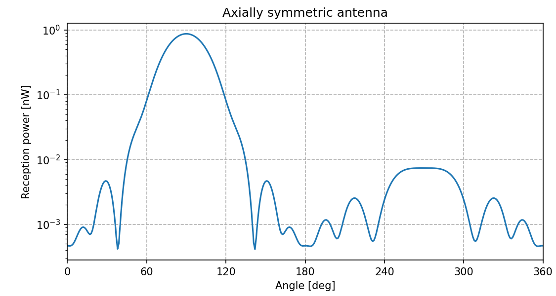
Here is the reception power vs. direction plot:
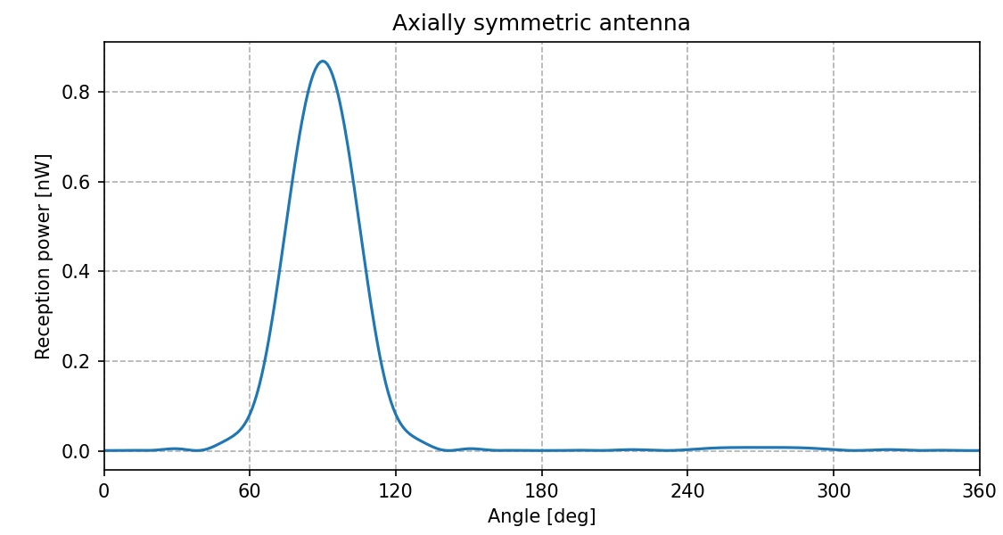
Here is the same plot with a logarithmic scale, where the details further from the main lobe are more apparent:
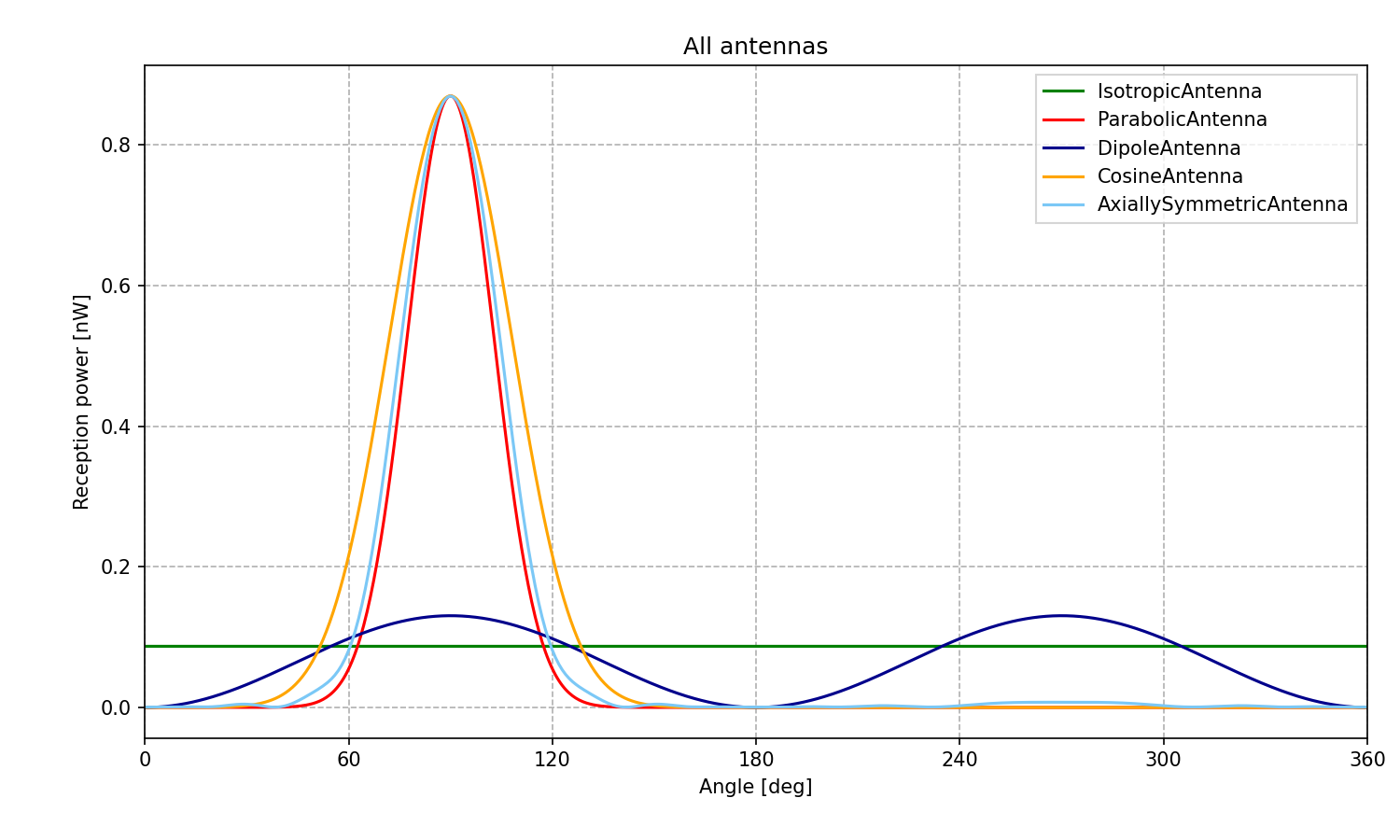
Here are the results for all antennas on one plot, for comparison:
Sources: omnetpp.ini, DirectionalAntennasShowcase.ned
Try It Yourself
If you already have INET and OMNeT++ installed, start the IDE by typing
omnetpp, import the INET project into the IDE, then navigate to the
inet/showcases/wireless/directionalantennas folder in the Project Explorer. There, you can view
and edit the showcase files, run simulations, and analyze results.
Otherwise, there is an easy way to install INET and OMNeT++ using opp_env, and run the simulation interactively.
Ensure that opp_env is installed on your system, then execute:
$ opp_env run inet-4.6 --init -w inet-workspace --install --build-modes=release --chdir \
   -c 'cd inet-4.6.*/showcases/wireless/directionalantennas && inet'
This command creates an inet-workspace directory, installs the appropriate
versions of INET and OMNeT++ within it, and launches the inet command in the
showcase directory for interactive simulation.
Alternatively, for a more hands-on experience, you can first set up the workspace and then open an interactive shell:
$ opp_env install --init -w inet-workspace --build-modes=release inet-4.6
$ cd inet-workspace
$ opp_env shell
Inside the shell, start the IDE by typing omnetpp, import the INET project,
then start exploring.
Discussion
Use this page in the GitHub issue tracker for commenting on this showcase.