Step 5. Taking interference into account
Goals
In this step, we make our model of the physical layer a little bit more realistic. First, we turn on interference modeling in the unit disc radio. By interference, we mean that if two signals collide (arrive at the receiver at the same time), they will become garbled and the reception will fail. (Remember that so far we were essentially modeling pairwise duplex communication.)
Second, we’ll set the interference range of the unit disc radio to be 500m, twice as much as the communication range. The interference range parameter acknowledges the fact that radio signals become weaker with distance, and there is a range where they can no longer be received correctly, but they are still strong enough to interfere with other signals, that is, they can cause the reception to fail. (For completeness, there is a third range called detection range, where signals are too weak to cause interference, but can still be detected by the receiver.)
Of course, this change reduces the throughput of the communication channel, so we expect the number of packets that go through to drop.
The model
To turn on interference modeling, we set the ignoreInterference
parameter in the receiver part of the GenericUnitDiskRadio module to false.
Interference range is defined by the interferenceRange parameter of
the GenericUnitDiskRadio module’s transmitter part, so we set that to 500m.
We expect that although host B will not be able to receive host A’s transmissions, those transmissions will still cause interference with other transmissions (e.g., R1’s) at host B.
Regarding visualization, we turn off the arrows indicating successful data link layer receptions because in our case, they do not add much value beyond displaying the network routes.
[Config Wireless05]
description = Taking interference into account
extends = Wireless04

*.host*.wlan[0].radio.receiver.ignoreInterference = false
*.host*.wlan[0].radio.transmitter.analogModel.interferenceRange = 500m

*.hostA.wlan[0].radio.displayInterferenceRange = true

*.visualizer.dataLinkVisualizer.packetFilter = ""
Results
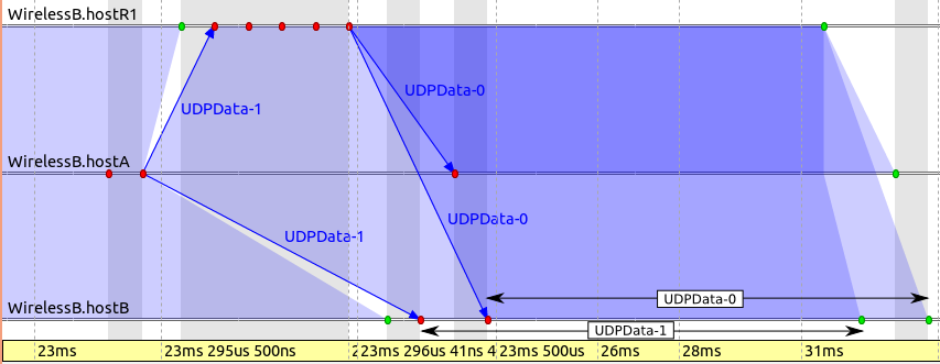
Host A is transmitting packets generated by its UDP Application module. R1 is at the right position to act as a relay between A and B, and it retransmits A’s packets to B as soon as they are received. Most of the time, A and R1 are transmitting simultaneously, causing two signals to be present at the receiver of host B, which results in collisions. When the gap between host A’s two successive transmissions is large enough, R1 can transmit a packet to B without collision.
When the packet UDPData-54 from host A arrives at host R1, it gets routed towards host B, so host R1 immediately starts transmitting it. Unfortunately, at the same time, host A is already transmitting the next packet (UDPData-55) back-to-back with the previous one. Thus, the reception of UDPData-54 from host R1 at host B fails due to a collision. The colliding packets are UDPData-55 from host A and UDPData-54 from host R1. This is indicated by the lack of appearance of a blue polyline arrow between host A and host B.
Luckily, the next packet (UDPData-56) from host A is not part of a back-to-back transmission. When it gets routed and retransmitted at host R1, there’s no other transmission from host A to collide with at host B. Interestingly, the first bit of the transmission from host R1 occurs just after the last bit of the transmission from host A. This happens because the processing, including the routing decision, at host R1 takes zero amount of time. The successful transmission is indicated by the appearance of the blue polyline arrow between host A and host B.
This is shown in the following animation:
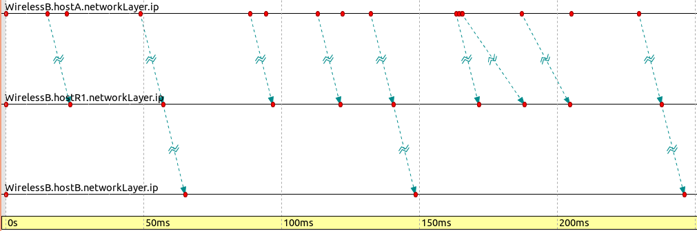
As expected, the number of packets received by host B is low. The following sequence chart illustrates packet traffic between hosts A, R1, and B’s network layer. The image indicates that host B only occasionally receives packets successfully; most packets sent by R1 do not make it to host B’s IP layer.
The following sequence chart shows host R1’s and host A’s signals overlapping at host B.
NOTE: On this and all other sequence charts in this tutorial, grey vertical strips are constant-time zones: all events within the same grey area have the same simulation time. Also, time is mapped to the horizontal axis using a nonlinear transformation so that both small and large time intervals can be depicted on the same chart. A larger distance along the horizontal axis does not necessarily correspond to a larger simulation time interval because the more events there are in an interval, the more it is inflated to make the events visible and discernible on the chart.
To minimize interference, some kind of media access protocol is needed to govern which host can transmit and when.
Number of packets received by host B: 183
Sources: omnetpp.ini,
WirelessB.ned
Discussion
Use this page in the GitHub issue tracker for commenting on this tutorial.