Wireless Signal Analog Domain Representations
Goals
Wireless signal analog domain representations are models that represent radio signals as physical phenomena as they are transmitted, received, and propagate in the wireless medium. Models of different complexity are available, suitable for different purposes.
In this showcase, we will describe the various analog signal representation models that are available and their advantages and drawbacks. We will also provide three example simulations that demonstrate the use of these models in typical use cases. By the end of this showcase, you will understand the different analog signal representation models and how they can be used to simulate the behavior of wireless systems.
4.6About Analog Models
The analog signal representation is a model of the signal as a physical phenomenon. Several modules take part in simulating the transmission, propagation, and reception of signals, according to the chosen analog signal representation model.
The transmission, propagation, and reception process is as follows:
The transmitter module creates an analog description of the signal
The analog model submodule of the radio medium module applies attenuation (potentially in a space, time, and frequency-dependent way).
The receiver module gets a physical representation of the signal and the calculated signal-to-noise-and-interference-ratio (SNIR) from the radio medium module.
The different types of transmitters, receivers and radio mediums each have a signalAnalogRepresentation parameter
to select one of the analog models.
INET contains the following analog model types, presented in the order of increasing complexity:
Unit disk: Simple model featuring communication, interference, and detection ranges as parameters. Suitable for simulations where the emphasis is not on the relative power of signals, e.g. testing routing protocols.
Scalar: Signal power is represented with a scalar value. Transmissions have a center frequency and bandwidth but are modeled as flat signals in frequency and time. Numerically calculated attenuation is simulated, and an SNIR value for reception is calculated and used by error models to calculate the reception probability.
Dimensional: Signal power density is represented as a 2-dimensional function of frequency and time; arbitrary signal shapes can be specified. Simulates time and frequency-dependent attenuation and SNIR. Suitable for simulating interference of signals with complex spectral and temporal characteristics and cross-technology interference (see also Coexistence of IEEE 802.11 and 802.15.4).
More complex models are more accurate but more computationally intensive.
INET contains a version of radio and radio medium module for each technology, e.g.
Ieee80211Radio / Ieee80211RadioMedium,
while the generic ApskRadio works with RadioMedium.
The analog model can be configured in radio and radio medium modules with the signalAnalogRepresentation parameter.
The analog model settings should match between the radios and the radio medium.
Here are some of radio types available in INET:
GenericRadio: simple radio model with parameters for bitrate, header length and preamble duration; contains GenericTransmitter and GenericReceiver
ApskRadio: a hypotetical radio that uses one of the well-known modulations without utilizing techniques such as forward error correction, interleaving, or spreading; contains ApskTransmitter and ApskReceiver
Ieee80211Radio: Wifi radio; contains Ieee80211Transmitter and Ieee80211Receiver.
Unit Disk Model
Overview
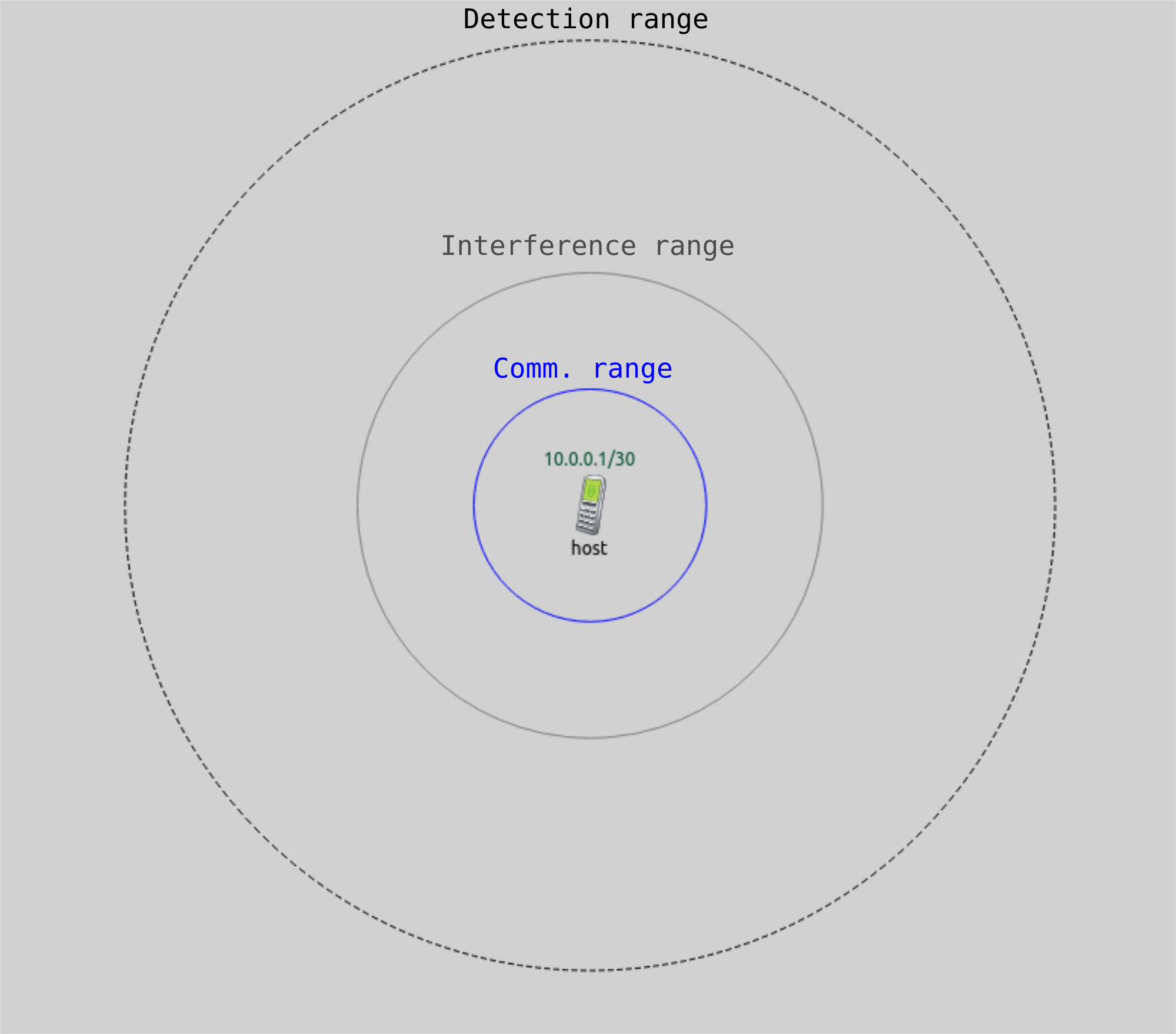
The unit disk analog model is the simplest available in INET. It models three ranges per radio, configurable with parameters:
Communication range: transmissions are always unsuccessful outside this range
Interference range: transmissions can’t interfere with and prevent other receptions outside this range
Detection range: transmissions can’t be detected outside this range; inside this range, transmissions might cause network nodes detecting them to defer from transmitting (when using a suitable MAC module, such as CsmaCaMac or Ieee80211Mac)
In general, the signals using any analog model might carry protocol-related meta-information, configurable by parameters of the transmitter, such as bitrate, header length, modulation, channel number, etc. The protocol-related meta-information can be used by the simulation model even with a unit disk, e.g. a unit disk Wifi transmission might not be correctly receivable because the transmission’s modulation doesn’t match the receiver’s settings.
Note
The simulated level of detail, i.e., packet, bit, or symbol-level, is independent of the used analog model representation, so as the protocol-related meta-infos on signals.
The unit disk receiver’s ignoreInterference parameter configures whether interfering signals
ruin receptions (false by default).
With the unit disk model, reception probability doesn’t change continuously with distance, but the change is abrupt at the edge of the communication range. Also, any interfering signal prevents reception, and obstacles completely block signals. There is no probabilistic error modeling.
The unit disk analog model is suitable for wireless simulations in which the details of the physical layer is not important, such as testing routing protocols (no detailed physical layer knowledge required). The unit disk model produces the physical phenomena relevant to routing protocols, i.e., varying connectivity; nodes have a range, transmissions interfere, and not all packets get delivered and not directly. In this case, it is an adequate abstraction for physical layer behavior.
All radios set to the unit disk analog model can be used with RadioMedium, just set the radio medium’s signal analog representation to unitDisk.
Example: Testing Routing Protocols
We’ll demonstrate the unit disk analog model in an example scenario featuring mobile ad hoc hosts, which use the AODV protocol to maintain routes:
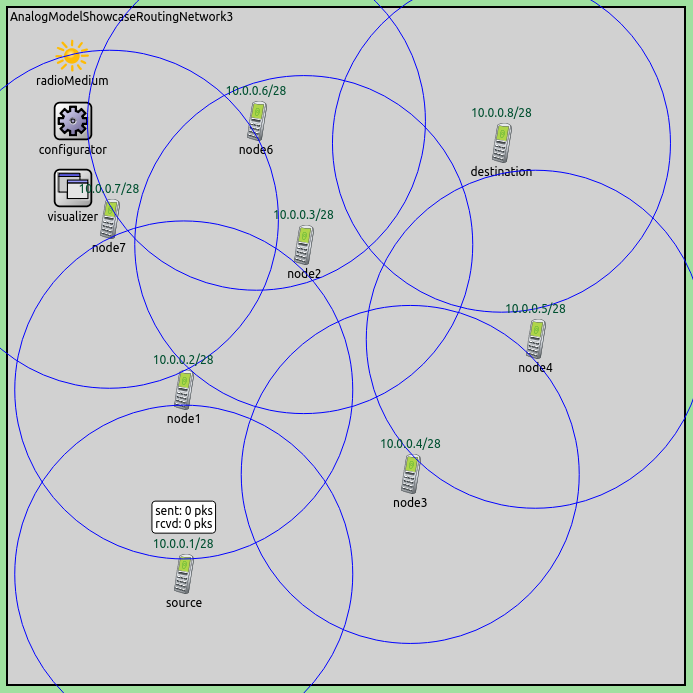
In the simulation, source sends ping requests to destination, and destination sends back ping replies.
The source and the destination hosts are stationary, the other hosts move around the scene in random directions.
The hosts use Ieee80211Radio, and the communication ranges are displayed as blue circles;
the interference ranges are not displayed, but they are large enough so that all concurrent transmissions
interfere. All hosts use the Ad hoc On-Demand Distance Vector Routing (AODV) protocol to maintain routes
as the topology changes so that they relay the ping messages between the source and the
destination hosts.
Here is the configuration in omnetpp.ini:
[Config Routing]
sim-time-limit = 5s
network = AnalogModelShowcaseRoutingNetwork

*.numHosts = 7

# ping app
*.source.numApps = 1
*.source.app[0].typename = "PingApp"
*.source.app[0].destAddr = "destination"

# node movement
*.node*.mobility.initFromDisplayString = false
*.node*.mobility.typename = "LinearMobility"
*.node*.mobility.initialMovementHeading = uniform(0deg,360deg)
*.node*.mobility.speed = 25mps

**.constraintAreaMaxX = 400m
**.constraintAreaMaxY = 400m
**.constraintAreaMinX = 0m
**.constraintAreaMinY = 0m

# routing
*.configurator.addStaticRoutes = false
**.netmaskRoutes = ""
*.*.routingApp.typename = "Aodv"
**.arp.typename = "GlobalArp"

*.*.routingApp.activeRouteTimeout = 1s
*.*.routingApp.deletePeriod = 0.5s

# radio
*.*.wlan[*].radio.signalAnalogRepresentation = "unitDisk"
*.radioMedium.signalAnalogRepresentation = "unitDisk"
**.radio.transmitter.analogModel.communicationRange = 200m
**.radio.transmitter.analogModel.interferenceRange = 400m
**.radio.transmitter.analogModel.detectionRange = 800m
**.displayCommunicationRanges = true
Here is a video of the simulation running (successful ping message sends between the source and destination hosts are indicated with colored arrows; routes to the destination are indicated with black arrows):
The source and destination hosts are connected intermittently. If the intermediate nodes move out of range before the routes can be built, then there is no connectivity. This can happen if the nodes move too fast since route formation takes time due to the AODV protocol overhead.
There is no communication outside of the communication range. Hosts contend for channel access, and defer from transmitting when there are other ongoing transmissions. The interference ranges of hosts cover the whole network, so transmissions cause interference all over the network.
Scalar Model
Overview
The scalar analog model represents signals with a scalar signal power, a center frequency, and a bandwidth. It also models attenuation and calculates a signal-to-noise-interference ratio (SNIR) value at reception. Error models calculate the bit error rate and packet error rate of receptions from the SNIR, center frequency, bandwidth, and modulation.
In the scalar model, signals are represented with a boxcar shape in frequency and time. The model can simulate interference when the interfering signals have the same center frequency and bandwidth and spectrally independent transmissions when the spectra don’t overlap at all; partially overlapping spectra are not supported by this model (and result in an error).
INET supports the scalar analog model in several radio and radio medium modules, such as IEEE 802.11, 802.15.4 and the generic ApskRadio.
The scalar model is more realistic than the unit disk model but also more computationally intensive. It can’t simulate partially overlapping spectra, only completely overlapping or not overlapping at all. It should be used when power level, attenuation, path and obstacle loss, SNIR, and realistic error modeling is needed.
Note
In showcases and tutorials, the scalar model is the most commonly used, it’s a kind of arbitrary default. When a less complex model is adequate in a showcase or tutorial, the unit disk model is used; when a more complex one is needed, the dimensional is chosen.
Example: SNIR and Packet Error Rate vs. Distance
In the example simulation, an AdhocHost sends UDP packets to another. The source host is stationary, the destination host moves away from the source host. As the distance increases between them, the SNIR decreases, and the packet error rate increases, as well as the number of successfully received transmissions.
Here is the configuration in omnetpp.ini:
[Config Distance]
sim-time-limit = 2.5s
network = AnalogModelShowcaseDistanceNetwork

**.radio.packetErrorRate.result-recording-modes = +vector
**.radio.bitErrorRate.result-recording-modes = +vector

# application parameters
*.source.numApps = 1
*.source.app[0].typename = "UdpBasicApp"
*.source.app[*].destAddresses = "destination"
*.source.app[*].destPort = 1000
*.source.app[*].messageLength = 1000byte
*.source.app[*].sendInterval = 1ms

*.destination.numApps = 1
*.destination.app[0].typename = "UdpSink"
*.destination.app[*].localPort = 1000

# mobility parameters
*.destination.mobility.typename = "LinearMobility"
*.destination.mobility.initialMovementHeading = 0deg
*.destination.mobility.speed = 100mps
*.destination.mobility.constraintAreaMinX = 500m
*.destination.mobility.constraintAreaMaxX = 825m

# wlan
*.source.**.transmitter.power = 5mW
*.source.**.displayCommunicationRange = true
**.backgroundNoise.power = -105dBm
**.wlan*.mac.*.rateSelection.dataFrameBitrate = 54Mbps
**.wlan*.mac.dcf.channelAccess.pendingQueue.packetCapacity = 14
The source host is configured to use the default 802.11g mode and 54Mbps data rate.
Here is a video of the simulation (successful link-layer transmissions are indicated with arrows; incorrectly received packets are indicated with packet drop animations):
As the distance increases between the two hosts, SNIR decreases, and the packet error rate increases, and packets are dropped. Note that the communication range of the source host is indicated with a blue circle. Beyond the circle, transmissions cannot be received correctly, and the signal strength falls below the SNIR threshold of the receiver. As an optimization, the reception is not even attempted, thus there are no packet drop animations.
Dimensional Model
Overview
The dimensional analog model represents signal power as a 2-dimensional function of time and frequency. It can:
Model arbitrary signal shapes
Simulate complex signal interactions, i.e., multiple arbitrary signal shapes can overlap to any degree
Simulate interference of different wireless technologies (cross-technology interference)
It is the most accurate analog signal representation, but it is computationally more expensive than the scalar model. In contrast to the unit disk and scalar models, the signal spectra of the dimensional analog model can also be visualized with spectrum figures, spectrograms, and power density maps (see Visualizing the Spectrum of Radio Signals).
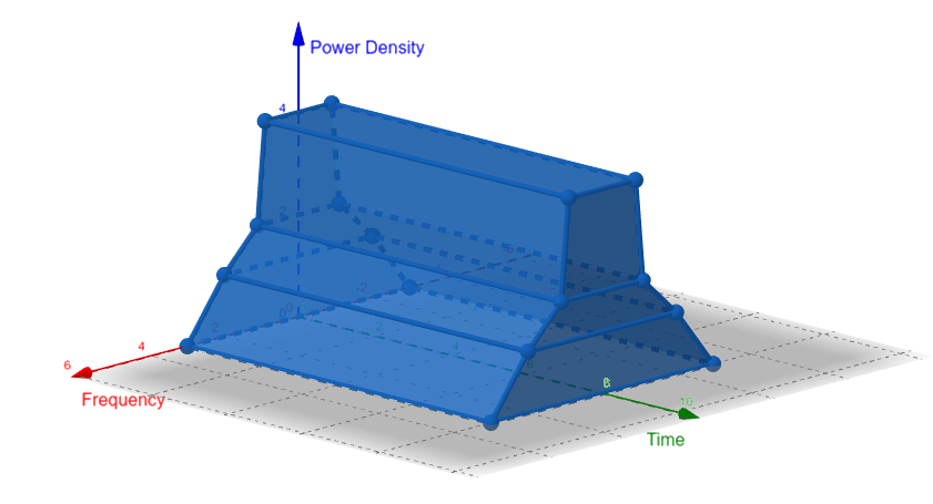
An example of a signal with a complex spectrum but constant in time
Note
When the dimensional model is used in a way equivalent to the scalar model (i.e., boxcar signal shape in frequency and time), its performance is comparable to the scalar’s.
The dimensional analog model uses an efficient generic-purpose multi-dimensional mathematical function API. The analog model represents signal spectral power density [W/Hz] as a 2-dimensional function of time [s] and frequency [Hz].
The API provides primitive functions (e.g., constant function), function compositions (e.g., function addition), and allows creating new functions, either by implementing the required C++ interface or by combining existing implementations. Here are some example functions provided by the above API:
Primitive functions:
Multi-dimensional constant function
Multi-dimensional unilinear function, linear in 1 dimension, constant in the others
Multi-dimensional bilinear function, linear in 2 dimensions, constant in the others
Multi-dimensional unireciprocal function, reciprocal in 1 dimension, constant in the others
Boxcar function in 1D and 2D, being non-zero in a specific range and zero everywhere else
Standard Gauss function in 1D
Sawtooth function in 1D that allows creating chirp signals
Interpolated function with samples on a grid in 1D and 2D
Generic interpolated function with arbitrary samples and interpolations between them
Function compositions:
Algebraic operations: addition, subtraction, multiplication, division
Limiting function domain, shifting function domain, modulating function domain
Combination of two 1D functions into a 2D function
Approximation in the selected dimension
Integration in the selected dimension
Interpolators (between two points):
Left/right/closer
Min/max/average
Linear/linear in decibel
The dimensional transmitters in INET use the API to create transmissions. For example:
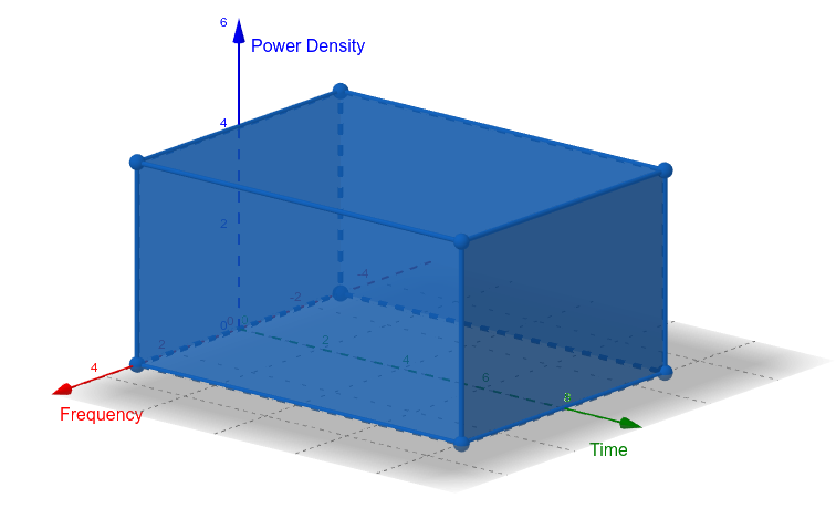
The 2D boxcar function is used to create a flat signal with a specific bandwidth and duration.
Transmission power is applied with the multiplication function.
The domain shifting function is used to position the signal on the frequency spectrum and to set it to the appropriate point in time.
Attenuation is also applied with the multiplication function (it’s more complicated, as attenuation is space, time, and frequency-dependent and takes obstacles into account).
Interfering signals are summed with the addition function.
SNIR is calculated by dividing the received signal by interfering signals.
Note
The above function composition can get really complex. For example, the medium visualizer uses a 5-dimensional function to describe the transmission medium total power spectral density over space (the whole scene), time (the whole duration of the simulation), and frequency (the whole spectrum). Similarly, the API can be used to create a space, time, and frequency-dependent background noise module (not provided in INET currently).
Note
The dimensional transmitters in INET select the most optimal representation for the signal, depending on the gains parameters (described later). For example, if the parameters describe a flat signal, they’ll use a boxcar function (in 1D or 2D, whether the signal is flat in one or two dimensions). If the gains parameters describe a complex function, they’ll use the generic interpolated function; the gains parameter string actually maps to the samples and the types of interpolation between them.
Several radios in INET, such as IEEE 802.11, narrowband and ultra-wideband 802.15.4, and APSK radio support the dimensional analog model.
The signal shapes in frequency and time can be defined with the frequencyGains
and timeGains parameters of transmitter modules. Here is an example signal spectrum definition:
**.frequencyGains = "left c-b*1.5 -40dB linear c-b -28dB linear c+b -28dB linear c+b*1.5 -40dB right"
Briefly about the syntax (applies to the timeGains parameter as well):
The parameter uses frequency and gain pairs to define points on the frequency/gain graph.
cis the center frequency andbis the bandwidth. These values are properties of the transmission, i.e. the receiver listens on the frequency band defined by the center frequency and bandwidth. However, the signal can have radio energy outside of this range, which can cause interference.Between these points, the interpolation mode can be specified, e.g.
left(take value of the left point),greater(take the greater of the two points),linear, etc.The
-inf Hz/-inf dBand the+inf Hz/-inf dBpoints are implicit (hence thefrequencyGainsstring starts with an interpolation mode).
Note
This is the mechanism that the transmitters in INET use to specify the signal shapes; there are multiple ways to specify signals, using the API.
The parameter value above describes the following spectrum (displayed on a spectrum figure):
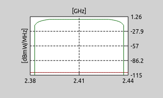
Note
Even though the interpolation between the points is linear, it appears curved due to the log scale used on the spectrum figure.
The timeGainsNormalization and frequencyGainsNormalization parameters set the normalization.
The normalization parameters specify whether to normalize the gain parameters in the given dimension
before applying the transmission power. The parameter values:
"": No normalization"integral": the area below the signal function equals 1"maximum": the maximum of the signal function equals 1
Then, the signal is multiplied by the transmission power.
Example: Interference of Signals with Complex Spectra
In the example simulation, there are two host-pairs; one host in each pair sends UDP packets to the other. The host pairs are on different, slightly overlapping Wifi channels. A noise source (NoiseSource) creates small bursts of noise periodically, which overlaps with all transmissions.
The NoiseSource module creates dimensional transmissions, which interfere with other signals. It contains a transmitter module (NoiseTransmitter), an antenna module (IsotropicAntenna by default), a mobility module (so that it has a position and can optionally move around):
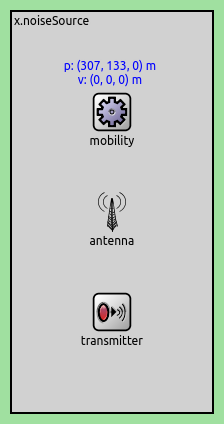
The noise transmissions don’t have any data or modulation, just a center frequency, bandwidth, power, and configurable arbitrary signal shape in frequency and time. It also has duration and sleep interval parameters.
Here is the configuration in omnetpp.ini pertaining to the radio settings:
*.host*.wlan[*].radio.signalAnalogRepresentation = "dimensional"
*.radioMedium.signalAnalogRepresentation = "dimensional"
*.host{1..2}.wlan[*].radio.channelNumber = 0
*.host{3..4}.wlan[*].radio.channelNumber = 3
*.host*.wlan[*].radio.transmitter.analogModel.frequencyGains = "left c-b*1.5 -40dB linear c-b -28dB linear c-b*0.5-1MHz -20dB linear c-b*0.5+1MHz 0dB linear c+b*0.5-1MHz 0dB linear c+b*0.5+1MHz -20dB linear c+b -28dB linear c+b*1.5 -40dB right"

*.noiseSource.transmitter.signalAnalogRepresentation = "dimensional"
*.noiseSource.transmitter.centerFrequency = 2500MHz
*.noiseSource.transmitter.bandwidth = 250MHz
*.noiseSource.transmitter.power = 0.0125W
*.noiseSource.transmitter.duration = uniform(0.1us, 0.5us) # bursts
*.noiseSource.sleepInterval = uniform(0.1ms, 0.5ms)

*.radioMedium.backgroundNoise.power = nan
*.radioMedium.backgroundNoise.powerSpectralDensity = -110dBmWpMHz
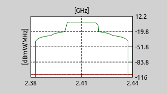
The hosts are configured to have Ieee80211Radio, with the analog model set to dimensional. The signal spectra
are configured to be the spectral mask of OFDM transmissions in the 802.11 standard.
Here is the spectrum displayed on a spectrum figure:
Note
In the current error models, the bit error rate is based on the minimum or mean of the SNIR, as opposed to per symbol SNIR.
Background noise is specified as power density, instead of power (specifying the signal strength with power is only relevant when the frequency of the signal is defined in a range).
The network looks like the following:
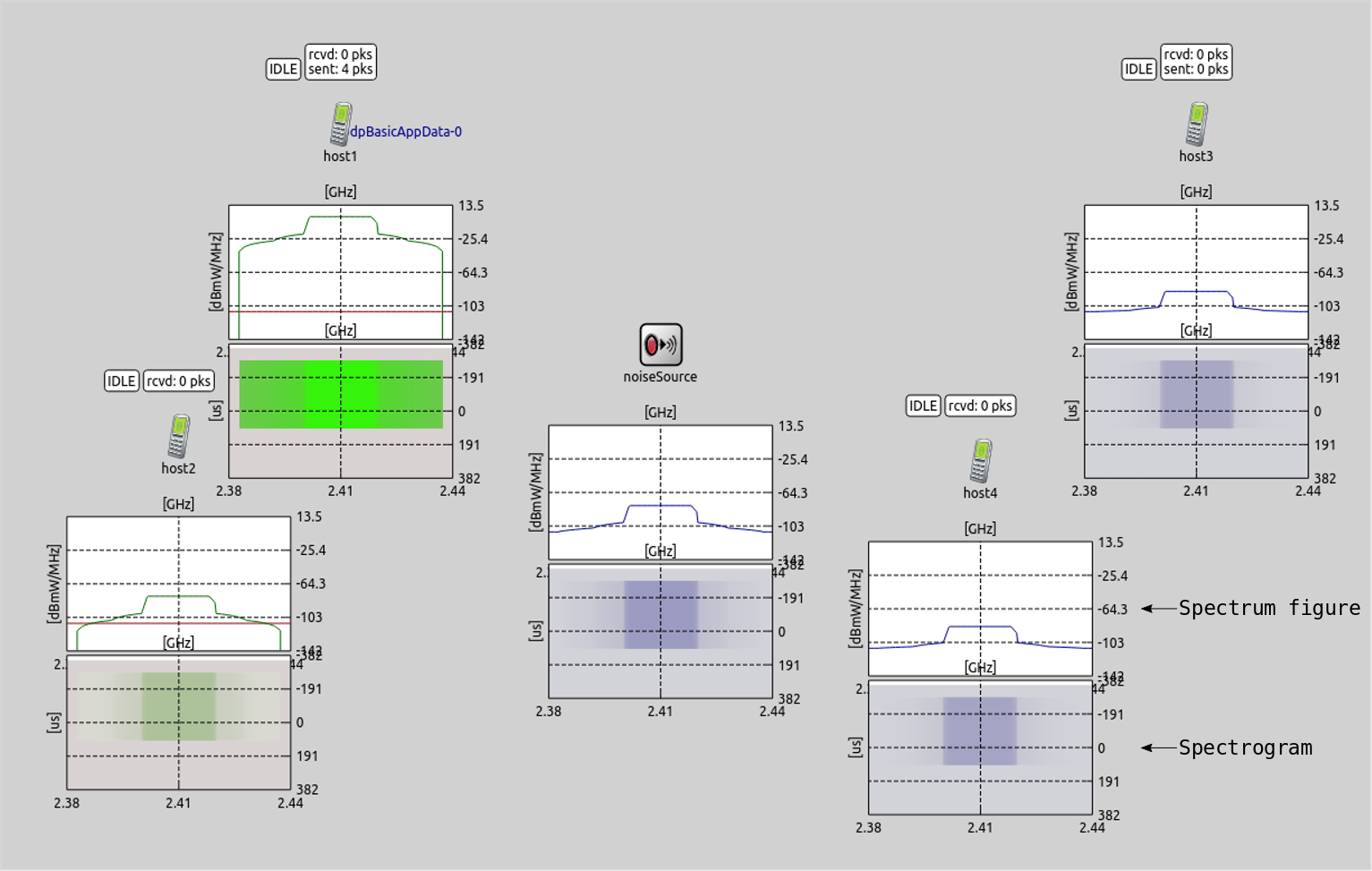
Here is a video of the simulation. Signals are visualized with colored rings, successful PHY and datalink-layer transmissions are visualized with arrows. The signals are displayed with spectrum figures and spectrograms:
Transmissions from one of the hosts and the noise source cause the other host to defer from transmitting. The noise transmissions often overlap the data frames, sometimes ruining reception. Note that the thin line of the noise on the spectrogram is much shorter than the data frame. Also, the spectrograms have a colored background due to the background noise (also displayed on the spectrum figures).
Sources: omnetpp.ini, AnalogModelShowcase.ned
Try It Yourself
If you already have INET and OMNeT++ installed, start the IDE by typing
omnetpp, import the INET project into the IDE, then navigate to the
inet/showcases/wireless/analogmodel folder in the Project Explorer. There, you can view
and edit the showcase files, run simulations, and analyze results.
Otherwise, there is an easy way to install INET and OMNeT++ using opp_env, and run the simulation interactively.
Ensure that opp_env is installed on your system, then execute:
$ opp_env run inet-4.6 --init -w inet-workspace --install --build-modes=release --chdir \
   -c 'cd inet-4.6.*/showcases/wireless/analogmodel && inet'
This command creates an inet-workspace directory, installs the appropriate
versions of INET and OMNeT++ within it, and launches the inet command in the
showcase directory for interactive simulation.
Alternatively, for a more hands-on experience, you can first set up the workspace and then open an interactive shell:
$ opp_env install --init -w inet-workspace --build-modes=release inet-4.6
$ cd inet-workspace
$ opp_env shell
Inside the shell, start the IDE by typing omnetpp, import the INET project,
then start exploring.
Discussion
Use this page in the GitHub issue tracker for commenting on this showcase.