Visualizing Radio Medium Activity
Goals
When simulating wireless networks, it can be useful to visualize the radio signals as they propagate through the environment. INET provides visualization features that make it easy to see which nodes are transmitting, which are receiving, and what signals are present at various points in the network.
This showcase consists of three simulation models that demonstrate the features of the radio medium activity visualizer, increasing in complexity from one model to the next.
4.6About the visualizer
The MediumVisualizer module (included in the networks for this showcase as part of IntegratedCanvasVisualizer) can visualize various aspects of radio communications. MediumVisualizer has the following three main features, and boolean parameters for turning them on/off:
Visualization of propagating signals: Signals are visualized as animated disks (
displaySignalsparameter)Indication of signal departures and arrivals: Icons are placed above nodes when a signal is departing from them or arriving at their location (
displaySignalDeparturesanddisplaySignalArrivalsparameters)Displaying communication and interference ranges: Ranges are displayed as circles around nodes (
displayCommunicationRangesanddisplayInterferenceRangesparameters)
The features above will be described in more detail in the following
sections. The scope of the visualization can be adjusted with parameters
as well. By default, all packets, interfaces, and nodes are considered
for the visualization. The selection can be narrowed with the
visualizer’s packetFilter, interfaceFilter, and nodeFilter parameters. Note that one
MediumVisualizer module can only visualize signals of one radio
medium module. For visualizing multiple radio medium modules, multiple
MediumVisualizer modules are required.
Displaying signal propagation, transmissions and receptions
In the example simulation for this section, we enable visualization of
propagating signals, displaying communication/interference ranges, and
signal departure/arrival indication. We demonstrate the visualization
with the visualizer’s default settings. The simulation can be run by
choosing the DisplayingPropagationTransmissionsReceptions
configuration from the ini file. The simulation uses the following
network:
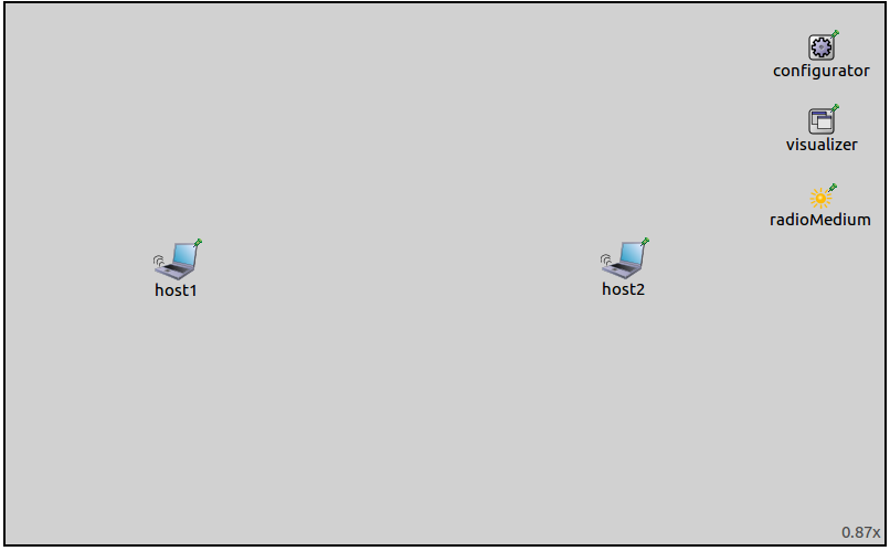
The scene size is about 900x600 meters. The network contains two
WirelessHost’s. host1 is configured to send UDP packets to
host2. Displaying of transmissions and receptions, propagating
signals, communication and interference ranges are enabled with the
following visualizer settings:
*.visualizer.mediumVisualizer.displaySignals = true
*.visualizer.mediumVisualizer.displayReceptions = true
*.visualizer.mediumVisualizer.displayTransmissions = true
*.visualizer.mediumVisualizer.displayCommunicationRanges = true
*.visualizer.mediumVisualizer.displayInterferenceRanges = true
When the simulation is run the network looks like this:
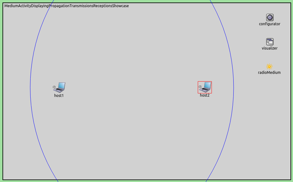
Parts of the communication range circles are visible in the image. With the current radio settings, the interference ranges are much larger than the communication ranges. One has to zoom out for them to be visible:
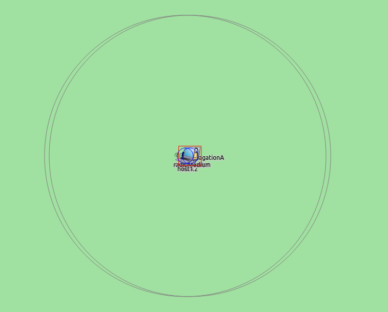
The communication and interference ranges are estimated for each node, from the node’s maximum transmitter power and the lowest receiver sensitivity setting in the network. The communication range represents the “best case” for signal reception (i.e. the range in which a signal would be correctly receivable by the most sensitive receiver in the network if the given node transmitted with its maximum transmitter power.) Transmissions are not correctly receivable beyond the communication range, but this does not imply that they are always correctly receivable in range. The interference range is similarly calculated from the maximum transmission power of the node, but it takes the minimum interference sensitivity level of all receivers in the network into account. As the communication range, the interference range is an estimation and means that signals beyond the interference range don’t cause reception errors due to interference (note that this is an optimization.)
The following video illustrates the visualization of propagating signals:
host1 sends an ARP request packet to host2, which sends an
ARP reply. host1 ACKs it, then sends the first UDP packet. This transmission
is followed by host2's ACK. The transmissions are visualized with
animated disks. The disk has an opacity gradient, which correlates with
the decrease in signal power as the distance from the transmitter
increases. The opacity indicates how strong the signal is compared to
the maximum power near the transmitter (but not compared to other
signals.) The blue signal departure indicator icons are displayed above
nodes when they are transmitting. Similarly, the red signal arrival
indicators are displayed above them when they are receiving. The
transmission power and power of the received signal is indicated on the
signal departure/arrival icons in dBW. Note that the signal arrival
indicator icon is displayed even when the receiving node cannot receive
the transmission correctly. (The signal arrival icons are placed above
nodes when there is a signal present at the location of the node. It
does not imply that the signal is receivable or that the node attempts
reception. Basically, the icon is displayed above all nodes that use the
same radio medium module.)
(The RadioVisualizer module can be used for displaying radio states, including when the radio is idle, sensing a signal, attempting reception, etc.)
The propagating signal
Regarding the visualization of radio signals, the density of interesting events varies on the simulation time scale. For example, we would like to visualize radio signals in a wifi network. The nodes are placed about 100 meters apart. When the signal starts propagating, it quickly reaches all nodes in the network, in about a few microseconds. The duration of the transmission is in the order of a few hundred microseconds (potentially up to milliseconds.) The visualizer changes the simulation speed, so that events that happen quickly don’t appear to be so fast as not to be observable (e.g. a signal’s edge propagating from a node), and other events that take longer on the timescale don’t appear to be slow and boring (e.g. the duration of a radio frame.) When there is a signal boundary (either at the beginning or the end of a transmission) traveling on the scene, the simulation is slowed down, and the rippling wave pattern is visible as the signal is propagating. When the signal is “everywhere” on the scene, i.e. its “first bit” has traveled past the farthest node, but its last bit has not been transmitted yet, the simulation is faster (the ripples are no longer visible, because of the increased simulation speed.)
The following three images illustrate that generally there are three different phases of signal propagation animation. The first is “expansion”; it starts when the signal’s “first bit” begins propagating from the transmitter node, and lasts until the “first bit” has traveled past the node farthest from the transmitter. In this phase, the simulation slows down. The second one is “presence”; it’s when the signal is “present” on the entire scene, at all nodes, and the simulation speeds up. The third one is “recession”; it starts when the signal’s “last bit” begins receding from the transmitter node, and lasts until the “last bit” has traveled past the farthest node. In this phase, the simulation slows down again. The transition between the two simulation speeds is smooth.

Also, it can happen that the simulation doesn’t slow down because the signal’s “last bit” gets transmitted before its “first bit” leaves the farthest node (basically, the signal looks like a thin ring.) Such a situation can happen if the transmission is very short, or if there are large distances between nodes, e.g. a few kilometers.
By default, the animation of all three phases has a duration of 1 second, wall clock time. Thus, as per the default settings, all signal propagation animations have a duration of 3 seconds, regardless of their actual simulated duration. To make the visualization more realistic, the visualizer’s animation speeds need to be set. When the animation speeds are set, the signal propagation animation becomes proportional to the transmission’s actual duration, thus transmission durations of packets can be compared (e.g. a smaller packet’s transmission animation takes less time than that of a larger packet.) The animation settings can be configured with the visualizer’s parameters, more on this in the next section.
Multiple nodes
This section describes the propagation animation settings of the
visualizer. The example simulation for this section contains three nodes
as opposed to two in the previous one, and the visualizer’s animation
speeds are specified for more realistic, proportional animation
durations. The example simulation can be run by choosing the
MultipleNodes configuration from the ini file.
Animation speed
The simulation speed during signal propagation animation is determined
by the visualizer’s animation speed parameters. The two parameters are
signalPropagationAnimationSpeed and
signalTransmissionAnimationSpeed (not specified by default). The
propagation animation speed pertains to the expansion/recession phase, i.e.
when a signal boundary is propagating on the scene. The
transmission animation speed refers to the presence phase, i.e. when no
signal boundary is visible. If no value is specified for these
parameters, the signalPropagationAnimationTime and
signalTransmissionAnimationTime parameters take effect. These
parameters set a fixed duration for the corresponding phases of the
transmission animation (this is the default setting, and both parameters
are 1 second). When the duration is fixed, all transmission animations
take the same amount of time, and NOT proportional to their actual
duration. A rule of thumb for setting the animation speed parameters is
given with the following example (assumes a wifi network with typical
node distances):
Setting the propagation animation speed to 300/c, where c is the speed of light, results in the animation speed value of 10^6, and the animation of the propagating signal traveling 300 meters on the scene in one second (when the playback speed is set to 1.)
The transmission animation speed should be about two magnitudes larger, as the time it takes for the propagating signal to reach the node farthest from the transmitter is two magnitudes smaller than the time it takes to transmit the signal. Thus in this example, it should be about 10^4.
The speed of the signal animation can be adjusted at runtime with the playback speed slider.
By default, the animation switches from the expansion phase to presence
phase when the propagating signal reaches the node farthest from the
signal source. The signalPropagationAdditionalTime parameter can
specify how long to continue the expansion/recession animation after the
edge of the signal has left the farthest node, to avoid flickering and
rapid changes in the animation.
The configuration
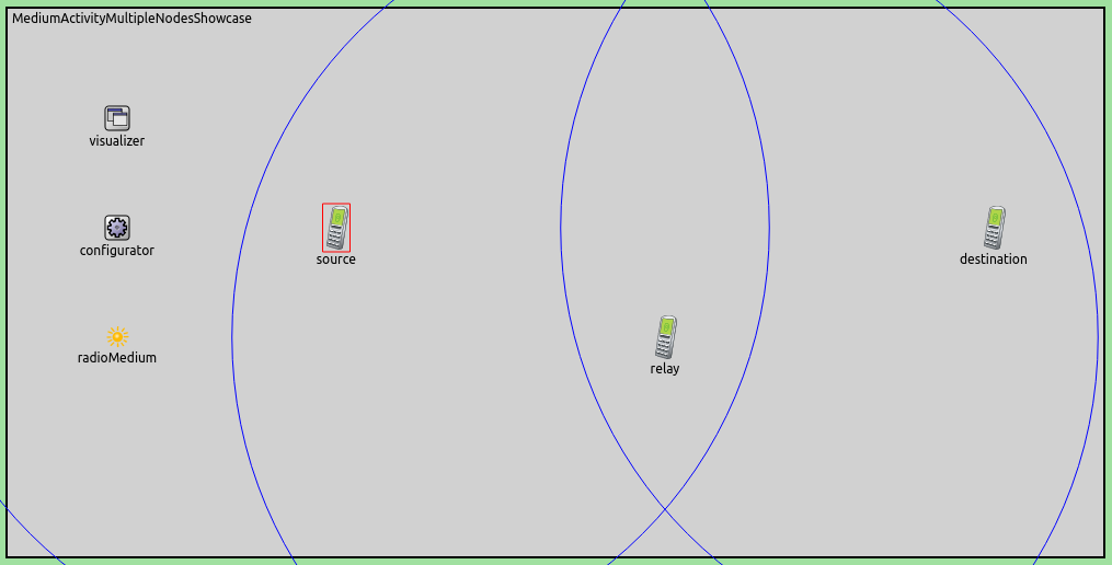
The example configuration for this section uses the following network:
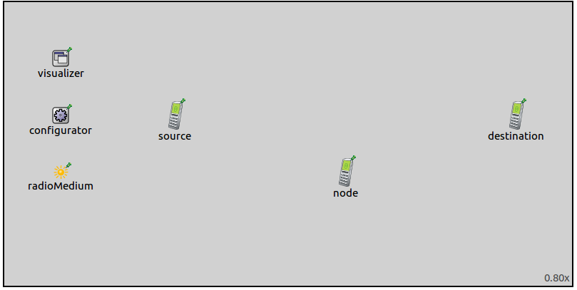
The scene size is 1000x500 meters. The network contains three
AdhocHost’s. The source is configured to ping the
destination. The communication ranges are configured so that hosts
can reach only the adjacent hosts. The center host is configured to
relay packets between the hosts on the two sides.
To demonstrate that the animation duration is proportional to the real
duration of the transmissions, relay is configured to use 24 Mbps
bitrate when transmitting, while the other hosts will use 54Mbps.
The visualizer’s configuration keys are the following:
*.visualizer.mediumVisualizer.signalPropagationAnimationSpeed = 500/3e8
*.visualizer.mediumVisualizer.signalTransmissionAnimationSpeed = 50000/3e8
*.visualizer.mediumVisualizer.displaySignals = true
*.visualizer.mediumVisualizer.displayTransmissions = true
*.visualizer.mediumVisualizer.displayReceptions = true
The visualization of propagating radio signals is turned on. The animation speed for the expansion and recession specified so that the expanding signal will travel 500 meters per second on the scene. The indication of signal departures and arrivals are also turned on. The communication and interference range circles are not enabled in this simulation; the following screenshot illustrates where the communication range circles would be if they were enabled:
When the simulation is run, this happens:
The video above depicts a UDP packet from source as it makes its way
to destination. When a node starts to transmit a frame, the
simulation is slower than during the propagation phase. As per the
parameters, the transmission travels 500 meters per second on the
scene. The animation durations of the transmissions are different
for certain packets. The UDP packet transmission from relay takes
more time than the one from source because of the different bitrate.
The transmission of the ACKs is the shortest because they are smaller than data
packets. (Even though they are transmitted with the slower
control bitrate, instead of data bitrate.)
Interfering signals
This configuration demonstrates how the visualization of interfering signals looks like. It uses the following network:

The scene size is 1000x500 meters. The network contains three
AdhocHost’s laid out in a chain, just like in the previous
configuration. The hosts on the two sides, source1 and source2,
are configured to ping the host in the middle, destination. There is
a wall positioned between the two hosts on the sides. The obstacle loss
model is IdealObstacleLoss, thus the wall blocks transmissions
completely. Both source hosts can reach the destination, but cannot
reach each other, and cannot detect whatsoever when the other source is
transmitting. Thus the collision avoidance mechanism can’t work
effectively.
Here is what happens when the simulation is run:
The two sources can’t detect each other’s transmissions, but they receive the ACKs and ping replies of the destination. Receiving these transmissions helps with collision avoidance, but the two sources often transmit simultaneously. When they do, both signals are present at the destination concurrently, visualized by the transmission disks overlapping. Since both sources are in communication range with the destination, the simultaneous transmissions result in collisions.
The simulation slows down whenever there is a signal boundary
propagating on the scene, even when there is also a signal with no
boundary present. Such is the case in the above video. source1
starts transmitting, and the signal edge is propagating. When it reaches
the farthest node, source2, the signal is present on the entire
scene, and the simulation speeds up. When source2 starts
transmitting, the simulation slows down again, although
source1’s signal is still present on the entire scene.
Generally, several signals being present at a receiving node doesn’t necessarily cause a collision. One of the signals might not be strong enough to garble the other transmission.
Sources: omnetpp.ini, RadioMediumActivityVisualizationShowcase.ned
More information
For further information, refer to the MediumVisualizer NED documentation.
Try It Yourself
If you already have INET and OMNeT++ installed, start the IDE by typing
omnetpp, import the INET project into the IDE, then navigate to the
inet/showcases/visualizer/canvas/radiomediumactivity folder in the Project Explorer. There, you can view
and edit the showcase files, run simulations, and analyze results.
Otherwise, there is an easy way to install INET and OMNeT++ using opp_env, and run the simulation interactively.
Ensure that opp_env is installed on your system, then execute:
$ opp_env run inet-4.6 --init -w inet-workspace --install --build-modes=release --chdir \
   -c 'cd inet-4.6.*/showcases/visualizer/canvas/radiomediumactivity && inet'
This command creates an inet-workspace directory, installs the appropriate
versions of INET and OMNeT++ within it, and launches the inet command in the
showcase directory for interactive simulation.
Alternatively, for a more hands-on experience, you can first set up the workspace and then open an interactive shell:
$ opp_env install --init -w inet-workspace --build-modes=release inet-4.6
$ cd inet-workspace
$ opp_env shell
Inside the shell, start the IDE by typing omnetpp, import the INET project,
then start exploring.
Discussion
Use this page in the GitHub issue tracker for commenting on this showcase.