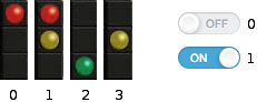
Instrument Figures¶

Goals¶

In complex simulations, there are usually several statistics that are vital for understanding what is happening inside the network. While these statistics can be found in the object inspector panel of Qtenv, they are not always easily accessible. INET provides a convenient way to display these statistics directly on the top-level canvas, through the use of instrument figures, which display various gauges and meters.

This showcase demonstrates the use of multiple instrument figures.

INET version: 4.1

Source files location: inet/showcases/visualizer/instrumentfigures

About Instrument Figures¶

Some of the instrument figure types available in INET are the following:

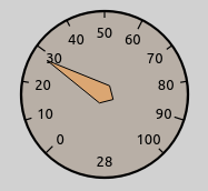
gauge: A circular gauge similar to a speedometer or pressure indicator.

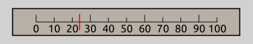
linearGauge: A horizontal linear gauge similar to a VU meter.

progressMeter: A horizontal progress bar.

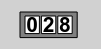
counter: An integer counter.

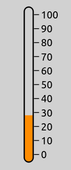
thermometer: A vertical meter visually similar to a real-life thermometer.

indexedImage: A figure that displays one of several images: the first image for the value 0, the second image for the value of 1, and so on.

plot: An XY chart that plots a statistic in the function of time.

The Network¶

The configuration for this showcase demonstrates the use of several instrument figures. It uses the following network:

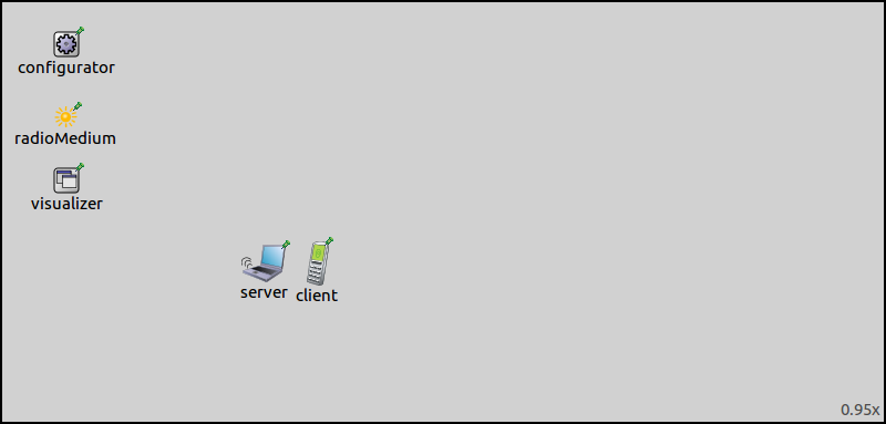
The network contains two AdhocHost nodes, a client and a server. (The visualizer is only needed to display the server’s communication range.) The scenario is that client connects to the server via WiFi, and downloads a 1-megabyte file. The client is configured to first move away from the server, eventually moving out of its transmission range, then to move back. Both hosts are configured to use WiFi adaptive rate control (AarfRateControl) so the WiFi transmission bit rate will adapt to the changing channel conditions, resulting in a varying application level throughput.

The Instruments¶

We would like the following statistics to be displayed using instrument figures:

Application level throughput should be displayed by a gauge figure, where throughput is averaged over 0.1s or 100 packets;
Wifi bit rate determined by automatic rate control should be displayed by a linearGauge figure and a plot figure;
Packet error rate at the client, estimated at the physical layer from signal-to-noise ratio, should be displayed by a thermometer figure and a plot figure;
The Wifi MAC channel access contention state of the server should be displayed by an indexedImage figure. IDLE means nothing to send, DEFER means the channel is in use, IFS_AND_BACKOFF means the channel is free and contending to acquire channel;
Download progress should be displayed by a progessMeter figure;
The number of socket data transfers to the client application should be displayed by a counter figure.

This is achieved by adding the following lines to the network compound module:

    @statistic[throughput](source=liveThroughput(client.app[0].packetReceived)/1000000; record=figure; targetFigure=throughputGauge; checkSignals=false);
    @figure[throughputGauge](type=gauge; pos=190,30; size=100,100; minValue=0; maxValue=25; tickSize=5; label="App level throughput [Mbps]");

    @statistic[bitrate1](source=server.wlan[0].mac.dcf.rateControl.datarateChanged/1000000; record=figure; targetFigure=bitrateLinearGauge);
    @figure[bitrateLinearGauge](type=linearGauge; pos=320,65; size=250,30; minValue=0; maxValue=54; tickSize=6; label="WiFi bit rate [Mbps]");

    @statistic[progress](source=100 * sum(packetBytes(client.app[0].packetReceived)) / 1048576; record=figure; targetFigure=progressMeter; checkSignals=false);
    @figure[progressMeter](type=progressMeter; pos=200,180; size=420,20; text="%.4g%%"; label="Download progress");

    @statistic[numRcvdPk](source=count(client.app[0].packetReceived); record=figure; targetFigure=numRcvdPkCounter; checkSignals=false);
    @figure[numRcvdPkCounter](type=counter; pos=760,260; label="Packets received"; decimalPlaces=4);

    @statistic[per1](source=packetErrorRate(client.wlan[0].radio.packetSentToUpper); record=figure; targetFigure=perThermometer);
    @figure[perThermometer](type=thermometer; pos=600,30; size=30,100; minValue=0; maxValue=1; tickSize=0.2; label="Packet error rate");

    @statistic[ctn](source=server.wlan[0].mac.dcf.channelAccess.contention.stateChanged; record=figure; targetFigure=ctnIndexedImage); // note: indexedImage takes the value modulo the number of images
    @figure[ctnIndexedImage](type=indexedImage; pos=800,340; size=32,32; images=showcases/idle,showcases/listen,showcases/clock; label="Contention state"; labelOffset=0,25; interpolation=best);

    @statistic[per2](source=packetErrorRate(client.wlan[0].radio.packetSentToUpper); record=figure; targetFigure=perPlot);
    @figure[perPlot](type=plot; pos=700,20; size=150,60; timeWindow=3; maxY=1; yTickSize=1; label="Packet error rate");

    @statistic[bitrate2](source=server.wlan[0].mac.dcf.rateControl.datarateChanged/1000000; record=figure; targetFigure=bitratePlot);
    @figure[bitratePlot](type=plot; pos=700,140; size=150,60; timeWindow=3; maxY=55; yTickSize=54; label="WiFi bit rate [Mbps]");

How does that work? Take the first one, throughputGauge, for example. Instrument figures visualize statistics derived from OMNeT++ signals, emitted by modules in the network. The source attribute of @statistic[throughput] declares that the client.app[0] module’s packetReceived signal should be taken (it emits the packet object), and the throughput() result filter should be applied and divided by 1000000 to get the throughput in Mbps. Further two attributes, record and targetFigure specify that the resulting values should be sent to the throughputGauge instrument figure. The next, @figure[throughputGauge] line defines the figure in question. It sets the figure type to gauge, and specifies various attributes such as position, size, minimum and maximum value, and so on.

Further details:

The gauge, linearGauge, and thermometer figure types have minValue, maxValue and tickSize parameters, which can be used to customize the range and the granularity of the figures.
The throughputGauge figure’s ticks are configured to go from 0 to 25 Mbps in 5 Mbps increments - the maximum theoretical application level throughput of WiFi “g” mode is about 25 Mbps. The application level throughput is computed from the received packets at the client, using the throughput result filter.
The bitrateLinearGauge figure’s ticks are configured to go from 0 to 54 Mbps in increments of 6, thus all modes in 802.11g align with ticks, e.g. 54, 48, 36, 24 Mbps and so on. The gauge is driven by the databitrate signal, again divided by 1 million to get the values in Mbps.
The perThermometer figure displays the packet error rate estimate as computed by the client’s radio. The ticks go from 0 to 1, in increments 0.2. It is driven by the packetErrorRate signal of the client’s radio.
There are two plot figures in the network. The perPlot figure displays the packet error rate in the client’s radio over time. The time window is set to three seconds, so data from the entire simulation fit in the graph. The bitratePlot figure displays the WiFi bit rate over time. Its value goes from 0 to 54, and the time window is 3 seconds.
The numRcvdPkCounter figure displays the number of data transfers received by the client. It takes about 2000 packets to transmit the file, thus the number of decimal places to display is set to 4, instead of the default 3. It is driven by the rcvdPk signal of the client’s TCP app, using the count result filter to count the packets.
The progressMeter figure is used to display the progress of the file transfer. The bytes received by the client’s TCP app are summed and divided by the total size of the file. The result is multiplied by 100 to get the value of progress in percent.
An indexedImage figure is used to display the contention state of the server’s MAC. An image is assigned to each contention state - IDLE, DEFER, IFS_AND_BACKOFF. The images are specified by the figure’s images attribute. Images are listed in the order of the contention states as defined in Contention.h file.

Running the Simulation¶

This video illustrates what happens when the simulation is run:

The client starts moving away from the server. In the beginning, the server transmits with a 54 Mbps bit rate. The transmissions are received correctly because the two nodes are close. As the client moves further away, the signal to noise ratio drops and packet error rate goes up. As packet loss increases, the rate control in the server lowers the bit rate, because lower bit rates are more tolerant to noise. When the client gets to the edge of the communication range, the bit rate is only 24 Mbps. When it leaves the communication range, successful reception is impossible, so the rate quickly reaches its lowest. After the client turns around and re-enters communication range, the rate starts to rise, eventually reaching 54Mbps again.

The download progress stops when the client is out of range since it is driven by correctly received packets at the application. Due to the reliable delivery service of TCP, lost packets are automatically retransmitted by the server. Thus the progress meter figure measures progress accurately.

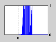
As the rate control changes the wifi bit rate, the application level throughput changes accordingly. The packet error rate fluctuates as the rate control switches between higher and lower bit rates back and forth. The following picture (a zoomed in view of the plot1 figure) clearly shows these fluctuations. It also shows packet error rate as a function of distance (due to constant speed).

Sources: omnetpp.ini, InstrumentShowcase.ned

Further information¶

For more information, refer to the Instrument Figures chapter of the INET User’s Guide.

Discussion¶

Use this page in the GitHub issue tracker for commenting on this showcase.